The application of Dempster-Shafer theory demonstrated with
justification provided by legal evidence
Shawn P.
Curley1
Department of Information & Decision Sciences
University of Minnesota
Judgment and Decision Making, vol. 2, no. 5, October 2007, pp. 257-276
Abstract
In forecasting and decision making, people can and often do represent
a degree of belief in some proposition. At least two separate
constructs capture such degrees of belief: likelihoods capturing
evidential balance and support capturing evidential weight. This
paper explores the weight or justification that evidence affords
propositions, with subjects communicating using a belief function in
hypothetical legal situations, where justification is a relevant goal.
Subjects evaluated the impact of sets of 1-3 pieces of evidence,
varying in complexity, within a hypothetical legal situation. The
study demonstrates the potential usefulness of this evidential weight
measure as an alternative or complement to the more-studied
probability measure. Subjects' responses indicated that weight and
likelihood were distinguished; that subjects' evidential weight tended
toward single elements in a targeted fashion; and, that there were
identifiable individual differences in reactions to conflicting
evidence. Specifically, most subjects reacted to conflicting evidence
that supported disjoint sets of suspects with continued support in the
implicated sets, although an identifiable minority reacted by pulling
back their support, expressing indecisiveness. Such individuals would
likely require a greater amount of evidence than the others to
counteract this tendency in support. Thus, the study identifies the
value of understanding evidential weight as distinct from likelihood,
informs our understanding of the psychology of individuals' judgments
of evidential weight, and furthers the application and meaningfulness
of belief functions as a communication language.
Keywords: belief functions, evidential weight, likelihood,
Dempster-Shafer theory, legal evidence.
1 Introduction
Probabilities are useful when acting in the absence of complete
knowledge, e.g., in forecasting or decision making. Such probabilities
are interpreted as measures of degrees of likelihood and are assessed
against a criterion of truth (von Winterfeldt & Edwards, 1986).
Scoring rules, as assessments of the quality of probability judgments,
operate from this perspective, comparing likelihood assessments to
actual outcomes, in an application of the truth criterion (see, e.g.,
Yates, 1990, chap. 3).
However, from the very origins of probability theory, scholars
recognized that truth is not the only criterion of potential interest
for interpreting probabilities. Smith, Benson and Curley (1991) tied
this recognition to a philosophical analysis of knowledge as
“justified true belief” (e.g.,
Shope, 1983) and to the use of probabilities as qualifications of
beliefs that fall short of knowledge. The analysis highlights two
separate criteria along which such beliefs may be qualified: truth and
justification. This theoretical distinction forms the basis of a
long-standing differentiation between Pascalian probability based on
likelihood relative to a criterion of truth and Baconian probability
based on support relative to a criterion of justification. (See Shafer,
1978, for an excellent historical discussion). The distinction is also
the basis of a common differentiation between the weight and the
balance of evidence that can be traced to Keynes (1921) and which has
played a major role in motivating the study of ambiguity in
decision-making beginning with Ellsberg (1961).
In short, likelihoods are intended to capture the balance of evidence
and are connected with the criterion of truth. If A is true, not-A is
false. To the degree that the evidence favors A, the balance of
evidence moves toward A and away from not-A in equal measure. The
weight of evidence is connected with the criterion of justification.
Weight depends upon the quantity and credibility of the evidence: How
much good evidence is there? How well does the evidence afford any
differentiation of possibilities?
Unlike evidential balance, evidential weight does not imply
complementarity. In probability theory, when the judgment of one
hypothesis increases, the sum of the judgments for the remaining
hypotheses must decrease by the same amount. In truth, one and only
one of a mutually exclusive set of events can occur, thus likelihoods
should exhibit complementarity, and probabilities capture this feature.
In contrast, evidential weight as a construct, grounded in the
criterion of justification, is not expected to exhibit this property.
Increased support for one possibility does not necessarily impinge on
the support for other possibilities. The belief functions of
Dempster-Shafer theory are discussed in this paper as
justification-based measures that do not incorporate complementarity as
a necessary axiom.
One source of the confusion between the constructs of likelihood and
weight, and of the measures attached to them, is that these constructs
and measures generally correlate. A useful analogy can be drawn here
with height and weight as two aspects of size. Though these measures
correlate, they capture distinct size constructs. Similarly,
probabilities as measures of likelihood and belief functions as
measures of justification may correlate, but they capture different
degree-of-belief constructs. Griffin and Tversky (1992) provided a
demonstration of the usefulness of the distinction, showing how the
inclusion of considerations of weight, in addition to the balance of
evidence, can serve to explain various empirical characteristics of
confidence judgments.
There are a number of situations in which justification is of primary
interest to the decision maker, or of interest in addition to truth.
For example, justification is of interest in legal settings (where the
goal is to remove doubt), in stock analysis (for which the emphasis is
upon justifying recommendations to clients), in diagnostic tasks in
which the truth is not feasibly determinable (e.g., within public
policy debates), and in scientific inference (cf. Ray & Krantz, 1996).
Despite this history and their potential usefulness, measures of
justification have been little studied empirically or been confounded
with measures of likelihood. The research has probably been somewhat
hampered by the respective and different natures of truth and
justification. Probability theory as capturing likelihoods benefits
from the ultimate realization of the truth in many instances for which
it is applied and because of the underpinnings of randomization and
relative frequency from which it historically derives (Curley, in
press; Hacking, 1975). The application of a system used for capturing
justification, and the use of Dempster-Shafer theory for this purpose,
is more equivocal about the underlying theoretical mechanisms
supporting such judgments (cf. Ray & Krantz, 1996; Shafer, 1976;
1981). Here the argument for applying Dempster-Shafer theory is based
on correspondence between aspects of evidential weight and unique
features of the theory, e.g., its noncomplementarity and the natural
representation of ignorance, i.e. the case where no information is
present (Curley & Golden, 1994).
In terms of previous work using Dempster-Shafer theory, most prior
research with this system has been theoretical, for example, in
pursuing the use of belief functions for propagating uncertainty in
AI/expert systems in addition or instead of using probabilities (e.g.,
Barnett, 1981; Cohen & Shoshany, 2005; Gillett & Srivastava, 2000;
Henkind & Harrison, 1988; Yang, Liu, Wang, Sii & Wang, 2006).
Although sparse, there is some suggestive empirical work. The cited
work of Griffin and Tversky (1992), directly, and the extensive work on
the effects of ambiguity in decision making (e.g., Camerer & Weber,
1992; Curley, Yates & Abrams, 1986; Einhorn & Hogarth, 1986; Hogarth
& Kunreuther, 1989), indirectly, testify to the relevance of
evidential weight to decision behavior. In addition, responses in
hypothetical legal contexts that emphasize justification exhibit
noncomplementarity of degrees of belief in a manner consistent with the
tenets of Dempster-Shafer theory (Curley & Golden, 1994; Schum &
Martin, 1987; van Wallendael & Hastie, 1990). Briggs and Krantz
(1992) adopted a measurement perspective and demonstrated that
judgments of evidential strength are separable. That is, subjects
“showed clear separation of relevant from irrelevant
evidence and of designated from surrounding relevant
evidence” (p. 77). In sum, the results support the
value and viability of measuring evidential weight as distinct from the
more commonly assessed construct of likelihood.
Since likelihood judgments have received more attention than weight
judgments and are often confused with them, particular emphasis must be
placed on this distinction. Specifically, important distinctions from
discussions in the literature need to be drawn: separating
justification-based measures such as in the present application of
Dempster-Shafer theory from weak theories of likelihood and from the
theory of subjective probability called Support Theory.
1.1 Important Distinctions
1.1.1 Weak Measures of Likelihood
With accumulating evidence that Expected Utility (EU) theory does not
provide an adequate descriptive theory of choice, one of the research
directions has been to investigate weaker theories of choice while
maintaining the expectation framework. Often this approach involves
relaxing or omitting one or more of the axioms that underlie EU theory
(e.g., as expressed by von Neumann & Morgenstern, 1947, or by Luce &
Suppes, 1965), or its close cousin Subjective Expected Utility (SEU)
theory (Savage, 1954). The use of weighting functions, like those in
Prospect Theory (Kahneman & Tversky, 1979; cf. Karmarkar, 1978) or in
Cumulative Prospect Theory (Tversky & Kahneman, 1992), exemplify an
approach in which a likelihood-based function in choice is modified to
accommodate subjects' behaviors that are incompatible
with EU and SEU.
It is important to recognize that belief functions are not being used
in this way. Although probability theory can be expressed
mathematically as a special case of belief functions (Shafer, 1976),
conceptually the two are distinct. Of interest are
subjects' expressions of justification, not of
likelihood. These are accepted as separate constructs. Belief
functions are not applied as a weaker measure of the same likelihood
construct that is captured by probability judgments. Belief functions
measure a separate construct with distinguishing features, e.g.,
noncomplementarity.
1.1.2 Support Theory
Support Theory has recently used a construct labeled “support” as a
building block of subjective probability (Rottenstreich & Tversky,
1997; Tversky & Koehler, 1994). This can easily lead to confusion
since the term has also been used to describe the construct of
evidential weight (notably by Shafer, 1976). However, as it has been
operationalized, Support Theory and the tasks to which it is applied
are clearly likelihood-driven. When Tversky and Koehler directly
assess “support” they do so by having subjects rate “the
[basketball] team you believe is strongest” (Study 3) and “the
suspiciousness of a given suspect” to a hypothetical crime (Study 4).
These ratings of cues that serve as the basis for subject's likelihood
judgments, as evidenced in their experiments, are not directly
equivalent to the support assessments within Dempster-Shafer theory
that are the subject of this paper.
These authors explicitly acknowledge this distinction of justification
and likelihood, and appropriately so, for example:
Judgments of strength of evidence, we suggest, reflect the degree to
which a specific body of evidence confirms a particular hypothesis,
whereas judgments of probability express the relative support for the
competing hypotheses based on the judge's general
knowledge and prior belief. The two types of judgments, therefore, are
expected to follow different rules. (Rottenstreich & Tversky, 1997,
p. 413)
There is a difference in the terminology: These authors use
“probability” and “relative support” to describe the
likelihood-based idea of balance, and use “strength of evidence” to
describe the justification-based idea of weight. Unfortunately, such
differences in terminology pervade the literature. Respectively,
Shafer (1976) distinguishes “chance” and “support,” Shafer and
Tversky (1985) distinguish “likelihood-based” or “Bayesian
designs” with “Jeffrey” or “belief-function designs.” In this
paper, I will generally use the terms of likelihood (truth, balance)
and evidential weight (justification, support). But, amidst the
terminology, the main point should not be lost. Support Theory is
likelihood-driven, defined relative to a criterion of truth.
Justification is a distinct criterion and measures of it have distinct
characteristics.
As also noted by Tversky and colleagues, justification-based weights,
in contrast to likelihood assessments, have been little studied. The
current paper, and the research stream within which it fits, serves to
fill this void. To operationalize the evidential weight construct, I
employ Dempster-Shafer theory, the best formulated system with features
appropriate for capturing evidential support in situations emphasizing
justification (Shafer, 1976; cf. Dempster, 1968).
The current study demonstrates an assessment approach grounded in
Dempster-Shafer theory as a basis for developing hypotheses. Curley
and Golden (1994), using similar though cruder methods, found that
nearly half of the subjects were able to consistently express beliefs
that qualitatively matched hypothesized expectations based on the
evidential content. Even subjects whose responses did not match the
expected pattern showed consistency in their use of the language,
supporting the coherence of people's use of belief
functions. Subjects also consistently responded in ways differing from
the prescriptions of probability theory, finding aspects of the belief
function language useful in expressing their beliefs. Golden (1993/4)
followed by examining the reliability (using a test-retest procedure)
and validity of subjects' responses in two studies.
With improvements in training, subjects showed even better qualitative
consistency than was observed by Curley and Golden. Numerically,
subjects also were able to respond reliably, though with room for
improvement, and the validity was high relative to the reliability.
Thus, the studies complemented the analysis of Briggs and Krantz (1992)
in supporting the viability of belief functions from a measurement
standpoint. Dempster-Shafer theory potentially offers a meaningful
response measure, particularly in a qualitative sense, that is distinct
from that of probability theory for use in investigating
subjects' degrees of evidential weight.
This paper demonstrates a technique using a measure from
Dempster-Shafer theory, applying it to sets of evidence that are
systematically constructed to get a fuller understanding of evidential
weight judgments from a psychological standpoint. The next section
provides a brief overview of Dempster-Shafer theory that serves as the
study's theoretical basis. Completing the paper are
four sections describing key features of evidential weight to be
investigated empirically, the methodology, the results, and a general
discussion, respectively.
1.2 Dempster-Shafer theory
Following is a brief description of elements of Dempster-Shafer theory
as it is applied here empirically. The theory is a system for
qualifying one's beliefs using numerical expressions
of degrees of support. Shafer (1976) provides a fuller theoretical
treatment for the interested reader.
Shafer described several, inter-related measures, conveying slightly
different messages about evidential weight, and the transformation
functions connecting them. One of these, Bel is termed a belief
function and is a commonly employed measure from the system. For
example, this is the measure used by Briggs and Krantz (1992). Here,
a different measure is elicited, the basic probability assignment, or
what I shall call the reserve function. Both measures capture a
degree of belief. The two measures have a 1–1 correspondence and are
mathematically inter-transformable, so the selection for assessment is
a matter of experimenter preference. The reserve function measure is chosen here
as being most conceptually like probabilities. Both probabilities and
reserve functions can be characterized as dividing the whole of one's belief (1.0)
into smaller elements. Consequently, the measure is believed to be an
intuitive one for individuals to assess. As noted, Briggs and Krantz
provide an empirical example using Bel, instead. Which of the two
measures might be better for assessment is an open empirical question
that is not addressed here. I do argue that the assessments
obtained in this study are meaningful and informative.
For brevity of exposition, hereafter belief is used
interchangeably with“degree of belief.”
Other terminology from the theory that is used in this paper includes:
Frame of discernment Θ:
A finite set of
possible values for a variable X, such that one, and only one, element
of the set is true. These elements are the possible states of nature
or hypotheses. In general, the items within the frame of discernment
develop as evidence accumulates, i.e., one can assign belief to Θ
without specifying what elements might be contained within it.
However, in this study for experimental control, the elements in the
frame are given to subjects, Θ = {a, b, c, d, e, f, g}.
Reserve Function:
This is the name given by Ray and Krantz
(1996, denoted as r in their paper) to
Shafer's “basic probability assignment,” and it is adopted here. This is a
non-negative, real-valued function, m, on the power set of Θ such
that:
(a) m(∅) = 0, where ∅ is defined as the null or impossible
event; and,
(b) Σ m(A) = 1, A ⊆ Θ.
The term reserve is borrowed from the idea of a contingency reserve in
budgeting, in which money is assigned to a category without specifying
how to divide it among the subcategories. Assigning m% of
one's belief to a subset in the power set of Θ
can be interpreted as: “Based on the evidence, I believe
with m% of my belief that the hypotheses in this set are supported;
however, I cannot distinguish between the elements in the set
individually.” Although this interpretation also holds
for m = 0, we use the term assign belief to signify that a
positive number is attached to a set. Also note that this function is
connected to, but distinct from, the belief function Bel defined by
Shafer:
Bel(B) = Σ m(A), for all A ⊆ B.
Singleton:
A subset of the power set of Θ that contains
only one element, e.g., {a}.
Simple support function:
A reserve function that assigns a
positive number to two and only two subsets of the power set, where one
of the subsets is Θ. All evidence used in the study was designed
to elicit simple support. The non-Θ subset for which the
evidence was designed to elicit positive belief is called the
target set of the evidence.
Multiple evidence requires an assessment of the joint impact of the
evidence. In a formal theory, like probability theory, this is
accomplished by a combination rule, like Bayes's
Theorem. In Dempster-Shafer theory, Dempster's Rule
is posited as a basis for assessing the joint impact of multiple
evidence.
Dempster's Rule:
A method for combining two
independent functions, m1 and m2, into
a new function, m:
m(A) = (1 - K)−1 Σ
m1(Ai)m2(Aj),
for all Ai ⊆ Θ, Aj
⊆ Θ
where Ai ∩ Aj = A; and
K = Σ m1(Ai)m2(Aj),
for all Ai ∩ Aj = ∅.
The parameter K is a measure of conflict in the
evidence.
The idea behind the combination rule is that initially your belief is
undifferentiated and allocated to Θ. As evidence becomes
available, you partition your belief into smaller subsets. This idea
is illustrated by Figure 1 for two pieces of evidence. Although shown
successively, Dempster's Rule is commutative, the order
of evidence is irrelevant. (See Golden, 1993/4, for evidence of
commutativity in subjects' assessments of evidential
weight and of a discussion of other properties of
Dempster's Rule and other proposed combination rules.)
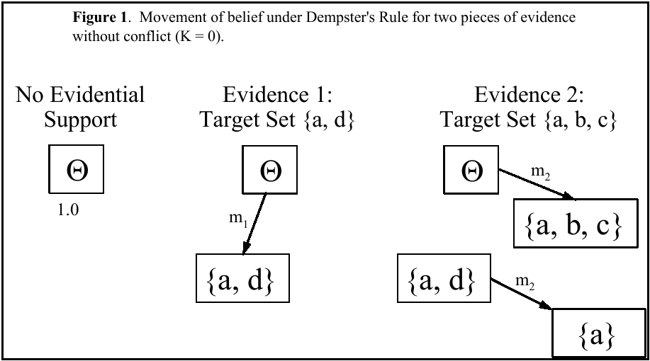
Initially, there is no evidence and all support (1.0) is in the
undifferentiated set Θ. As shown, the first piece of evidence
implicates a and d, not differentiating between them. The function
m1 moves a portion of the weight of evidence into the
set {a, d} to convey this, leaving the remainder of the weight in the
set Θ. How much weight is moved depends on the reliability,
credibility and strength of the evidence. The second piece of evidence
implicates a, b and c. The function m2 moves a portion
of the weight from Θ into {a, b, c} and moves the same
proportion of the weight from {a, d} to the intersection of the two
sets: {a}. In this way, as evidence accumulates, support becomes
differentiated into finer subsets capturing the justification for the
possible evidential conclusions.
1.3 Key Aspects of Evidential Weight
We form beliefs in response to evidence; we assign degrees of belief to
the extent that the evidence is not definitive. The present study
demonstrates psychological aspects of subjects'
judgments of evidential weight using systematically created sets of
evidence. Key characteristics for analysis in the assessment of
justification are identified in this section.
1.3.1 Inconclusiveness
As noted earlier, an important difference between likelihood and
support is the noncomplementarity of evidential weight. If the
evidence does not justify A, this does not necessarily imply
justification for not-A. Instead, the evidence may be silent with
respect to either. For example, if evidence of questionable
reliability supports A, we would qualify the justification it provides
for A based on the evidence's unreliability. We would
not, however, then transfer the remainder of its justification to
not-A. To the extent the evidence is unreliable, it does not implicate
either A or not-A.
Relatedly, the representation of ignorance has been a controversial
topic in the use of probability theory (e.g., DeGroot, 1970; Winkler,
1972). Having a natural means of expressing ignorance, by assigning
belief to the superset Θ may prove to be an attractive, intuitive
feature of belief functions. The degree of belief m(Θ)
represents one's undifferentiated belief that is
withheld in complete reserve, expressing nonsupport for any subset of
possibilities, e.g., due to evidential unreliability.
If individuals view inconclusiveness as a meaningful aspect of support,
then a sensible and persistent use of m(Θ) should be observed.
First, since the evidence in the study is inconclusive, subjects should
generally assign belief to Θ to communicate this. Second, as
evidence accumulates and becomes more conclusive, m(Θ) should
decrease. Not all theories of support have this latter property. For
example, Dubois and Prade (1986) proposed an averaging rule in which
the m(Θ) of combined evidence is proposed to be intermediate to
the m(Θ) of the individual pieces of evidence. This rule
corresponds to a leveling of support rather than a focusing of support
as the underlying psychology in accumulating support.
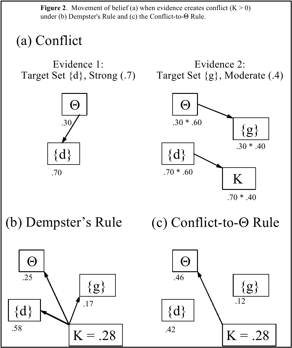
Another key issue in understanding justification is the reaction to
evidential conflict. Consider Figure 2, showing an example of support
with conflicting evidence. Evidence 1 provides simple support for
{d}. It is fairly strong evidence, though inconclusive with
m1(d) = .70.2 Evidence 2 is of more moderate
strength and implicates {g} with m2(g) = .40.
Clearly, the evidence is conflicting, implicating disjoint sets of
possibilities. Applying Dempster's Rule for
independent pieces of evidence, the resulting weight of conflict is K =
.28 (Figure 2a).
Two general possible reactions are that one can react to conflict with
continued confidence in the evidence or by pulling back support.
Formal rules corresponding to each of these psychological reactions
have been proposed. The rules receiving best support in a preliminary
study (Golden 1993/4) are highlighted here, and represent these two
divergent psychological approaches to conflict. The rules are not
claimed as descriptive in the sense that individuals are presumed to
perform the calculations of the combination rules. However, as
capturing different approaches to conflict, the rules provide useful
standards of comparison for contrasting the underlying psychological
theories.
Dempster's Rule exemplifies a rule capturing continued
confidence in the evidence by distributing conflict proportionally into
already implicated sets (Figure 2b). Following this normalization,
m(Θ) = .25, less than both m1(Θ) = .30 and
m2(Θ) = .60. It is easily shown that these
strict inequalities will hold whenever the evidence is inconclusive,
mi(Θ) > 0 for i = 1, 2. The
attitude is one of: “I know there is conflict, but
my beliefs are still sound, just not focused yet.”
Since Dempster's Rule does embody implicit claims
about how people assign evidential weight, other researchers have
questioned these claims and proposed alternative combination schemes.
One alternative is a Conflict-to-Θ Rule (Yager, 1987). The rule
operates like Dempster's Rule, except when there is
conflict, K > 0. Instead of normalizing, the rule assigns
all of K to Θ, as shown by Figure 2c. Thus, the rule captures
indecisiveness as the psychological reaction to conflict. The attitude
is one of: “The conflict indicates that I do not know
what is happening. It reflects indeterminacy and my ignorance. Thus,
I should pull my belief back into Θ.” For this
rule, in the example, the combined m(Θ) = .46 after adjustment.
In this case, the value is greater than m1(Θ) =
.30. Although, this does not necessarily happen, we see here that the
rule allows the possibility of greater indecisiveness with increasing
evidence, in marked contrast to the attitude embodied in
Dempster's Rule.
Golden (1993/4) reported evidence that subjects in aggregate behaved
midway between Dempster's Rule and the
Conflict-to-Θ Rule, with no support for other tested rules. The
present study allows an individual-level analysis to investigate how
individual subjects react to conflict.
1.3.3 Simplification
Evaluating evidence becomes increasingly complex as evidence
accumulates, even more so in assessing justification than likelihood.
For belief functions the possible number of assessments increases
exponentially with the number of distinct alternatives. For example,
if Θ contains seven separable alternatives, then no more than
seven probability assessments are needed, but as many as
(27 - 1) = 127 positive reserve numbers (values of m)
may be applied. Thus, the number of values can quickly exceed the
capacity of an individual to maintain information in working memory
(Miller's, 1956, 7 ± 2).
Given the limitation, subjects likely will simplify their reserve
functions with the accumulation of evidence of differing implications.
However, subjects should do so in a reasoned, not haphazard, manner,
maintaining main lines of implication while truncating others. Of
interest is this purposiveness as it exists: What strategies do
individuals employ to simplify the lines of justification without
sacrificing important information?
In sum, the study demonstrates the use of belief functions, using the
reserve function form, for communicating evidential weight, while
addressing three psychological concerns:
-
How do subjects communicate inconclusiveness?
- How do subjects react to conflict, particularly do they
tend to show continued confidence in the evidence or pull back support?
- How do subjects simplify complex evidential weight?
The study addresses these questions using an established task and
systematically varied sets of evidence. The more extensive evidence
sets also allow individual-level analyses, affording the possibility of
identifying individual differences in behavior with respect to these
questions.
2 Method
2.1 Subjects
Sixty-six non-law graduate students at the University of Minnesota
voluntarily participated in the study. The subjects engaged in a
juror-type task, evaluating evidence in a hypothetical legal setting
and requiring no special law experience. They were paid a fixed fee
for participating in a single session lasting less than two hours.
Each subject was in the session individually with a single
experimenter.
Table 1: Hypothetical situation to which subjects responded
Bensten Murder Case
Your Task: You have been asked to help the county attorney assess
evidence gathered by police in a murder case. The county attorney
would like you to evaluate the evidence and state how you believe the
evidence implicates the seven suspects. The county attorney may or may
not have more evidence, but at this time the county attorney is only
interested in examining the effects of the following pieces of
evidence. The county attorney asks that the evaluation be done for the
pieces of evidence individually, as well as collectively, because the
county attorney is unsure which suspect will be charged and which
evidence will be used in court. Your analysis will be used to guide
the on-going police investigation and to help the county attorney in
the pre-trial preparation of a case. At this time the police are sure
of a couple of things: 1) the murderer acted alone, and 2) the list of
suspects is complete.
The Crime: On Monday, the 20th of April, Thomas Bensten was found
murdered in his 3rd floor Edina office suite. Mr. Bensten is a 45 year
old single executive for a company named PSV Enterprises. Mr.
Bensten's body was discovered at approximately 6 a.m.
by one of the building's janitors. The janitor was
unlocking the building's doors as part of his job.
The police arrived shortly after 7 a.m. and concluded that Mr. Bensten
had been murdered with a 44 caliber handgun. The gun had been shot
into Mr. Bensten's left shoulder at close range after
what appears to have been a significant struggle. The time of death
was set between 7 p.m. Friday, April 17th and 11 a.m. Saturday, April
18th.
2.2 Procedure
The experimental procedure began with a training session that provided
subjects with instruction in the language of reserve functions. The
Appendix contains the full training materials. These materials were
similar to those employed by Golden (1993/4); and, the training case
was similar to the experimental case. It involved the same task as
described in Table 1, but for a different crime description — an auto
theft. Aside from familiarizing the subjects with the task, the
training instructed subjects in the vocabulary of the belief function
language. That is, given a belief, how could a subject express this
belief in the theory's language? And conversely,
given a reserve function, what does it communicate? The order and
content of training involved instructions about:
-
The task (Table 1)
- What it means to assign belief to a set of suspects,
e.g., selecting the set {B, D} “represents your
belief that either Suspect B or Suspect D is guilty, but based on the
evidence, you cannot differentiate this belief between the two
suspects.”
- The response form (Table 2), demonstrated for single
pieces of evidence
- Seven examples pairing text descriptions of beliefs with
the belief functions that communicate these descriptions.
- Practice case, Part 1: The subject responded to four
individual pieces of evidence for an auto theft case similar to the
upcoming experimental case.
- Practice case, Part 2: The subject responded to four
pairs of evidence for the auto theft case.
The subjects were not schooled in any particular form of reserve function, and were
informed that there was no right or wrong belief given the evidence.
They also were not instructed in any particular way of combining
evidence when responding to more than one piece of evidence. Golden
(1993/4) used a post-training quiz to check subjects'
understanding after training. All subjects (total N = 64) achieved
sufficient mastery, so the quiz was not employed in the current study.
Table 2: Sample response area.
| Evidence #1 |
Sets
|
Strength
|
| |
|
| |
|
| |
|
| |
|
| |
|
| |
|
| |
|
Total
(must add to 1)
|
|
Following the training, subjects read a page describing the
hypothetical situation to which the evidence related and the role that
they were to take in responding to the evidence (Table 1). Each
subject then responded in succession to 18 single pieces of evidence, 4
evidence pairs and 17 evidence triples. The pairs and triples were
constructed using items from the 18 single pieces of evidence. The
stimuli are described below.
Subjects first received a stimulus booklet containing the 18 single
pieces of evidence, each on a separate page. They responded to each
piece of evidence in turn and in isolation, separately from all
preceding evidence. Each single evidence was numbered consecutively,
and the responses were recorded on a separate response booklet. In
providing their responses, subjects were advised during the training to
first identify which sets should be assigned belief and then to assign
the numerical beliefs to these sets. Thus, the qualitative assessment
of identifying the implicated sets preceded and was separate from the
quantitative assessment.
After completing the first stimulus booklet, the subjects received a
second stimulus booklet with the four evidence pairs (which appeared
first) and the 17 evidence triples . For the pairs and triples,
stimuli and response forms were in the same booklet. Evidence used in
the stimuli were numbered to match the numbering used in the
single-evidence booklet. Subjects could refer back to their
single-evidence response booklet to check their responses while going
through the pairs and triples booklet. This capability was described
during the training.
After completing the second booklet, subjects were debriefed and paid.
2.3 Stimuli
Subjects responded to single pieces, pairs, and triples of evidence.
The structure by which the evidence sets were constructed is now
described.
Table 3: Brief descriptions of the contents of the individual pieces of evidence
used in the study along with the mean (standard deviation) belief
attached to the target set for that evidence.
Motive Evidence
.54 (.25) Suspect being Blackmailed by victim
.41 (.25) Suspect recently Fired from Job by victim
.38 (.26) Suspect felt Cheated in a Business Venture with
victim
.35 (.26) Suspect in victim's Will
.30 (.22) Recent Argument with victim
.30 (.23) Violent Personality indicated by psychological
testing
Opportunity Evidence
.52 (.29) Suspect had Pass Key to the building
.52 (.32) No Alibi from another for time of crime
.40 (.31) Suspect with previously registered .44 caliber
Handgun (gun unavailable)
Physical Evidence
.83 (.19) Blood type match
.64 (.28) Fingerprints (partial); possible match with suspect
.61 (.28) Left-Handed Stab Wound; left-handed suspect
.55 (.30) Foot Print (partial); possible match with suspect
.46 (.33) Aspirin Bottle at scene; suspect not under
doctor's orders to avoid aspirin
.43 (.30) Cigarette Ashes; suspect smoked cigarettes
.34 (.29) Nonprescription Sunglasses at scene; suspect does not
have either prescription or contact lenses
.24 (.27) Glasses of untouched Scotch at scene;
suspect drinks alcohol
.21 (.23) Valuable Baseball missing (otherwise no valuables
taken); suspect is baseball fan
Note: N = 66 subjects for each mean and standard deviation.
2.3.1 Single evidence
The materials were adapted from those tested by Curley and Golden
(1994) and Golden (1993/4). Table 1 describes the experimental
situation and the subjects' assigned role. Subjects
saw 18 single pieces of evidence. Table 3 contains brief descriptions
of the content of the 18 pieces of evidence. Subjects saw paragraph
descriptions of each. For each piece of evidence, subjects received
information for each of the seven possible suspects. They responded
using a response table like that in Table 2. The information was
constructed to provide simple support, implicating a single target set
of suspects. For example, the following piece of evidence (Fired from
Job) provides support for target set {a, b, e}:
Some of the suspects had been recently fired from PSV Enterprises by
Mr. Bensten. The reason Mr. Bensten gave for the firings was that the
employees had inadequate quality of work. The firings cost each of the
men approximately $40,000.
| Suspects |
Recently Fired by Mr. Bensten |
| Suspect A |
Yes |
| Suspect B |
Yes |
| Suspect C |
No |
| Suspect D |
No |
| Suspect E |
Yes |
| Suspect F |
No |
| Suspect G |
No |
Each subject saw each of the 18 pieces of evidence in Table 3 and saw
evidence implicating 18 target sets. The pairing of target sets to
evidence content was randomized, and the order of evidence presentation
was also randomized.
The single pieces of evidence were selectively combined into sets of
evidence containing two or three pieces of evidence.
(3,2)
(0.15,1.75)(a) Identical
(.5,1.4).53
(.5,1.4).45
(.45,1.35)d
(1.65,1.75)(b) Embedded
(2,1.4)1.2
(2,1.4).25
(1.78,1.35)a
(1.97,1.35)d
(0.15,.85)(c) Intersecting
(.35,.5).5
(.65,.5).5
(.2,.47)e
(.45,.47)a
(.75,.47)f
(1.65,.85)(d) Disjoint
(1.65,.5).5
(2.3,.5).5
(1.6,.47)d
(2.25,.47)g
2.3.2 Evidence Pairs
For two pieces of evidence, there are four possible combination forms
associated with target sets, disregarding the order of evidence and
specific evidence content. The target sets for the two pieces of
evidence may be either identical, embedded, intersecting, or disjoint.
Examples of each are given and illustrated in Figure 3:
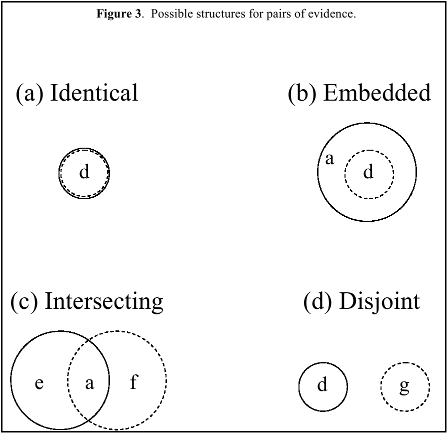
The particular target sets were also selected so that each of the
regions in Figure 3 contains a single suspect. Each subject responded
to one of each of these structures, involving eight separate single
pieces of evidence from among those seen earlier.3 Recall that the content of the evidence items was randomly
varied across subjects. Presentation order of the pair structures was
also randomized.
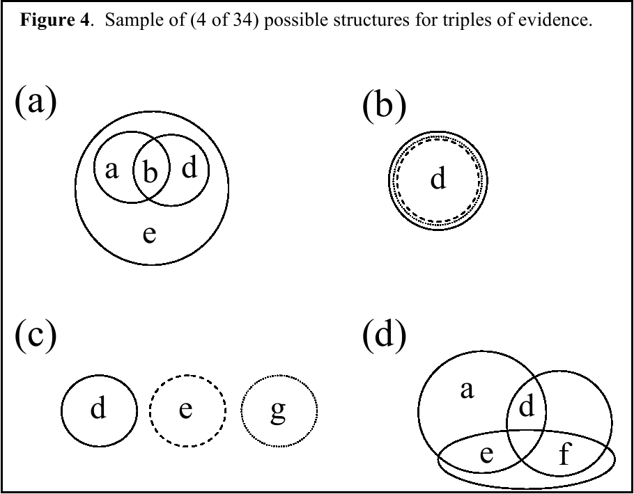
2.3.3 Evidence Triples
For three pieces of evidence, there are 34 possible combination forms,
disregarding evidence order and specific content. Testing all of these
combinations requires 18 separate pieces of evidence (which led to the
selection of the 18 used as single pieces of evidence). Again,
evidence content and presentation order were randomized. Also, to stay
within a reasonable time frame for a single session, each subject saw
17 evidence triples. Selection of 17 of 34 triples was randomized so
that each of the 34 triple structures was assessed by 33
subjects.4 (The use of 66
subjects was motivated by this randomization design.)
Examples of four of the evidence triple structures are given and
illustrated in Figure 4.
Again, note that the particular target sets were selected so that each
of the regions in Figure 4 (and for all other triple structures)
contains a single suspect.
3 Results
3.1 Validity
All single pieces of evidence seen by subjects were designed to provide
simple support. The degree to which subjects perceived the evidence in
terms of simple support can be used as a qualitative measure of
structural validity, i.e., a meaningfulness measure which does not rely
on the numerical responses but simply on the sets that are assigned
belief — the qualitative structure of the responses. Overall, 95%
(1123/1188, 18 pieces of evidence × 66 subjects) of responses to
single pieces of evidence were structurally valid, assigning belief
only to the target set and/or Θ. This exceeds the 59% found by
Curley and Golden (1994) and is comparable to the 92% and 96% found
in the two experiments reported by Golden (1993/4). From a
methodological perspective, the comparisons indicate: (a) the
improvement in training materials after the first empirical effort by
Curley and Golden, and (b) the success in streamlining the training
materials after Golden's study without loss of
meaning. Unlike Curley and Golden, there were no consistent
non-structurally valid response patterns. In particular, subjects did
not respond with consistent use of the complement of the target set or
consistent use of non-target singletons.
Thus, subjects saw evidence as effecting a movement of support into the
implicated set. The subjects did not overextend this support into
smaller subsets than was warranted by the evidence or into sets that
were not directly implicated. They also did not reply in a way
mimicking probability assessment (though such a function was seen
during training, see Example #5 in the Appendix).
Table 3 shows the mean beliefs assigned to the target set for the
content of each of the individual pieces of evidence. As to numerical
validity, the orderings of the means are reasonable relative to the
content of the evidence. There are no obvious misalignments in the
data.
3.2 Inconclusiveness
There was a high use of Θ across all subjects. For single pieces
of evidence and evidence pairs, 91% of the reserve functions assigned
belief to Θ. For the evidence triples, 77% of the responses
assigned positive belief to Θ. Overall, mean m(Θ) declined
as evidence accumulated from .53 for singles (n = 1188, s = .32) to .32
for pairs (n = 264, s = .27), and .20 for triples (n = 1122, s = .23).
Subjects commonly used this ability to communicate that the evidence as
a whole was not conclusive. Inconclusiveness is an evidential weight
concept, not available in probability assessment, that was meaningful
to the subjects.
As a cleaner view of this tendency, consider responses to accumulating
evidence in favor of a single target element: for a single piece of
evidence, the evidence pair in Figure 3a, and the evidence triple in
Figure 4b. For these responses, the mean m(Θ) declined with
accumulating evidence from 0.53 to 0.31 to 0.21. Individually, of the
33 subjects responding to the triple in Figure 4b, 22 (67%) decreased
m(Θ) from single to pair and from pair to triple. This tendency
is consistent with the claim of theories like
Dempster's Rule and the Conflict-to-Θ Rule. In
contrast, only 1/33 (3%) responded consistently with an averaging
approach both to the evidence pair and to the evidence triple, giving a
cumulative response that was intermediate to the component single
evidence responses in both cases.
3.3 Conflict
In considering methods of combining the support provided by multiple
evidence, we distinguish situations that involve conflict from those
that do not. One pair of evidence (66 responses) and fourteen triples
(458 responses = 14 × 33 subjects/triple, with 4
missing5) involved structural conflict. To compare
subjects' responses, focus is on the weight attached
to Θ. It is in the assignment to Θ that the rules most
markedly differ in a way that is informative of how the respondents
reacted to that conflict (Figure 2).
Overall, in response to conflicting evidence,
subject's mean m(Θ) = .27. From applying
Dempster's Rule to the responses for the single pieces
of evidence, the expected mean m(Θ) = .25. From applying the
Conflict-to-Θ Rule to the responses for the single pieces of
evidence, the expected mean m(Θ) = .44. These means suggest a
closer correspondence of aggregate behavior with
Dempster's Rule. Of the 524 total m(Θ)
responses, 297 were closer to the value predicted by
Dempster's Rule whereas 121 were closer to the value
predicted by the Conflict-to-Θ Rule (the remainder were
equidistant). Thus, the single best descriptive model in the aggregate
is provided by Dempster's Rule.
However, a better picture of how subjects handled support in the face
of conflict arises from individual-level analyses that are possible
with the current design. The distribution of the m(Θ) responses
relative to the predictions from the two rules as applied to the
responses for single pieces of evidence is shown in Table 4.
Table 4: Distribution of m(Θ) responses
relative to the predictions from the two rules for single pieces of
evidence.
| (a) |
219 responses: |
m(Θ) < |
Dempster's Rule |
|
|
| (b) |
121 responses: |
|
Dempster's Rule |
< m(Θ) < |
Conflict-to-Θ Rule |
| (c) |
127 responses: |
|
|
|
Conflict-to-Θ Rule < m(Θ) |
| (d) |
35 responses: |
m(Θ) = |
Dempster's Rule |
< |
Conflict-to-Θ Rule |
| (e) |
4 responses: |
|
Dempster's Rule |
< |
Conflict-to-Θ Rule = m(Θ) |
| (f) |
18 responses: |
m(Θ) = |
Dempster's Rule |
= |
Conflict-to-Θ Rule |
Thus, although the aggregate response is intermediate to the two rules,
fully 2/3 of the responses are more extreme than either rule, with 219
responses expressing even more conclusiveness than
Dempster's Rule, and 127 expressing less
conclusiveness than the Conflict-to-Θ Rule.
Further individual-level analysis suggests two identifiable subgroups
of individuals. For the analysis, each of the 524 responses was
categorized as in one of the six categories labeled (a)-(f) above.
For each subject, I then asked whether the subject had a modal response
category among (a)-(f) with which he or she responded consistently at
a greater than chance rate (binomial test using one-tailed α =
.05). Of 66 subjects, 25 could be classified as having a consistent
response pattern; the
distribution of these subjects relative to the two rules is:
| (a) |
10 subjects: |
m(Θ) < Dempster's Rule |
| (b) |
7 subjects: |
Dempster's < m(Θ)
< Conflict-to-Θ |
| (c) |
8 subjects: |
Conflict-to-Θ Rule < m(Θ) |
Groups (a) and (c), those with the lowest and highest m(Θ),
both had more significant (p<.05) results than would be expected by
chance, 10 and 8, respectively, out of 56, when the expectation would
be about 3. In fact, they had significantly more such results, by a
binomial test (p<.01 for both). This result suggests that
individual differences were real. The mean (standard deviation)
values for m(Θ) for the three groups are:
(a) .29 (.25)
(b) .16 (.12)
(c) .56 (.23).
In comparison, the mean (standard
deviation) values of m(Θ) as predicted from applying Dempster's
Rule to the single evidence responses are:
(a) .41 (.26)
(b) .10 (.12)
(c) .37 (.26).
Thus, the 17 subjects responding below (Group a) and just above (Group
b) Dempster's Rule are behaving similarly and qualitatively like
Dempster's Rule. These subjects reliably react to conflict by
continuing to move their support downward into the implicated subsets.
Those behaving below (Group a), as opposed to above (Group b),
Dempster's Rule basically differ in being less conclusive in their
responses to the single pieces of evidence. That is, those subjects
who were more extreme in moving evidence downward away from Θ
compared to Dempster's Rule (Group a) were less conclusive with single
pieces of evidence (as indicated by a higher m(Θ) applying
Dempster's Rule). Those subjects who were less extreme in moving
evidence downward from Θ compared to Dempster's Rule (Group b)
were more conclusive in their responses to single pieces of evidence
(as indicated by a lower m(Θ) applying Dempster's Rule). This
latter group may be showing a floor effect: Having largely moved
belief away from Θ for the single pieces of evidence (mean
m(Θ) = .10), there was little room to further move belief from
Θ with multiple pieces of evidence (mean m(Θ) = .16).
But, the main point is that subjects in both Groups (a) and (b)
reacted similarly to conflict: They tended to react with continued
confidence in the evidence even with conflict, similarly to how
Dempster's Rule operates.
In contrast, the eight subjects who reliably responded with an
m(Θ) at the high end (Group c) behaved qualitatively more like
the Conflict-to-Θ Rule. They responded similarly to Group (a)
subjects for single pieces of evidence, but they reacted differently
under conflict. For the Group (c) subjects, conflict led to
indecisiveness. Faced with conflict, they tended to withhold their
belief, as expressed by their increasing support to Θ.
3.4 Simplification
As evidence accumulates, its evaluation becomes increasingly complex.
Given the well-established cognitive limitations of humans to deal with
the resultant complexity in all its detail, some means of
simplification is cognitively desirable. And, as humans are adaptive,
it is believed that subjects simplify in a sensible, not haphazard,
manner.
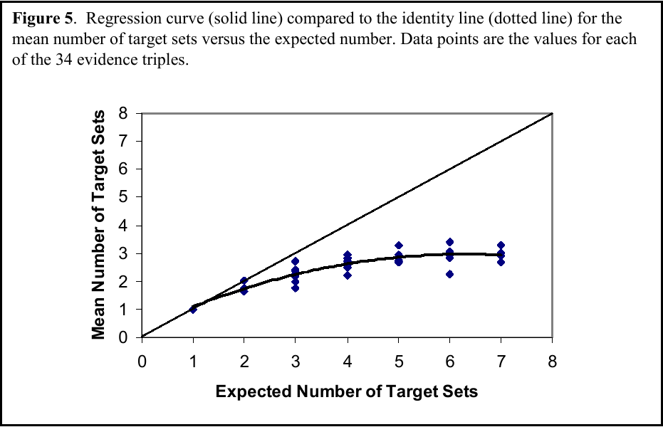
An overall view of whether subjects simplified their lines of
implication is provided by Figure 5 in an analysis of
subjects' responses to triples of evidence, where
complexity is likely to be present if at all. For a given evidence
structure, some number of sets are expected to get positive belief
aside from Θ. The expected number of target sets implicated by
the evidence ranges from 1 to 7 for the different structures of
evidence triples used in the study, as shown on the x-axis. For
example, the triple in Figure 4a has four expected target sets:
{a,b,d,e}, {a,b}, {b,d}, and {b}. On the y-axis is the mean,
across subjects, of the actual number of sets that are assigned belief
for each of the 34 triple structures used in the study. A quadratic
regression model shows significant curvature, with the quadratic
coefficient β2 being less than zero. This same
quadratic pattern appears in analyses of the data from individual
subjects. For the individual analyses, H0:
β2 ≥ 0, for the quadratic model, is
rejected at the 0.05 level for 57/66 subjects and at the 0.10 level for
61/66 subjects.
Basically, what the analyses support is a simplification of lines of
implication, reducing the number of sets receiving support compared to
theoretical expectations. Subjects are somehow focusing their
attention to certain lines of implication while truncating others. It
is now of interest to investigate the logic of the simplification
through analysis for sets of differing cardinality and the use of
singletons.
3.4.1 Cardinality
A general overview of how simplification is happening arises from
viewing the distribution of subjects' beliefs across
sets of different cardinality. The number of elements in a target set
can range from 1 to 7, e.g., the target set {a,b,d,e} has four
elements and Θ has 7 elements. Table 5 displays how subjects
distributed their belief across the possible set sizes when responding
to three pieces of evidence. The table compares responses for evidence
triples to expectations based on applying Dempster's
Rule to the single evidence responses. Overall, the subjects moved
their belief into sets of size 1, i.e., singletons. They used fewer
sets of sizes 2–4 and assigned less belief to these set sizes than
would be expected from Dempster's Rule. This pattern
of response was mainly observed when there was no structural conflict
in the evidence.
Table 5: Mean belief attached and numbers of subjects attaching positive belief
to sets of differing cardinalities, by subjects and by application of
Dempster's rule: overall, and with and without Structural Conflict.
| |
Sets of Size: |
| 2-8 |
1 |
2 |
3 |
4 |
5 |
6 |
7 (Θ) |
| Overall |
|
|
|
|
|
|
|
| Actual |
.58 |
.17 |
.12 |
.12 |
.19 |
.14 |
.23 |
| Nactual |
967 |
421 |
219 |
93 |
23 |
09 |
865 |
| Dempster's Rule |
.41*** |
.31*** |
.21*** |
.16* |
.09 |
.15 |
.23 |
| NDempster |
995 |
847 |
495 |
193 |
16 |
13 |
898 |
| Npaired1 |
1079 |
899 |
571 |
244 |
39 |
20 |
989 |
| Conflict cases |
|
|
|
|
|
|
|
| Actual |
.55 |
.18 |
.17 |
.15 |
.17 |
.06 |
.23 |
| Nactual |
355 |
138 |
95 |
25 |
11 |
03 |
330 |
| Dempster's Rule |
.53 |
.25*** |
.16 |
.08 |
.10 |
.14 |
.20** |
| NDempster |
408 |
270 |
162 |
29 |
12 |
10 |
321 |
| Npaired |
411 |
301 |
207 |
49 |
23 |
12 |
368 |
| Non-conflict cases |
|
|
|
|
|
|
| Actual |
.59 |
.17 |
.09 |
.11 |
.22 |
.31 |
.24 |
| Nactual |
579 |
271 |
120 |
67 |
12 |
06 |
508 |
| Dempster's Rule |
.32*** |
.34*** |
.25*** |
.19*** |
.06 |
.07 |
.25 |
| NDempster |
555 |
548 |
333 |
164 |
04 |
02 |
550 |
| Npaired |
635 |
569 |
360 |
194 |
16 |
07 |
591 |
| 1Sample sizes for use of the paired differences test,
t(n-1), comparing actual mean belief for the evidence triple to the
mean belief predicted by applying Dempster's Rule to
the single evidence responses. Only responses with positive values for
either the actual or predicted belief are included in this
analysis. |
| * p < .05; ** p < .01;
*** p < .0001. |
Thus, subjects have a tendency to move their support into singletons as
much as possible, particularly when there is no conflict in the evidence.
(The individual differences in patterns of behavior under conflict have
already been discussed above.) This greater use of singletons
parallels the application of a likelihood measure like probability
theory that applies belief only to
singletons. Therefore, further investigation of how the subjects assign
support to singletons is of particular interest.
3.4.2 Singletons
As a first look, we can isolate for each structure every singleton
that received positive belief from at least one subject. Some of
these are target singletons, i.e., singletons that were expected to
receive belief based on the structure of the evidence. (For example,
for the triple illustrated by Figure 4a, {b} is a target singleton,
and for the triple in Figure 4d, {d}, {e}, and {f} are target
singletons.) All target singletons for all evidence triples received
belief. Other, non-target singletons also sometimes received belief.
Table 6a shows the mean evidential weight ( m )
across all subjects and singletons, for each singleton that received
positive belief in response to evidence triples. The means are
separated between target and non-target singletons. The means are
also separated by the number of pieces of evidence in the triple that
implicated the element in the singleton. As an example, for the
triple in Figure 4d, the sets {d}, {e}, and {f} are target
singletons and are each implicated by two pieces of evidence, e.g.,
{d} is implicated by {a, d, e} and {d, f}. For this triple,
eight subjects also assigned positive belief to {a}. This is a
non-target singleton implicated by one piece of evidence: {a, d, e}.
As expected, higher weight is attached to singletons which are
implicated by more evidence. This effect is particularly pronounced
for target singletons. The same increasing pattern also obtains for
the numbers of subjects who assign belief to the singletons (Table 6b).
More subjects assign more evidential weight to singletons implicated
by more evidence. Subjects are identifying and placing support upon
the target elements.
Another interesting result was that, primarily, only two types of
singletons received positive belief across the variety of evidence
structures shown to subjects. The first type was a target singleton as
noted above. Of the possible target singletons across all subjects and
evidence sets, 70% received positive belief as expected. All 66/66
subjects used at least one target singleton in their responses. When
the evidence pointed to a particular possibility, subjects identified
this and focused belief on this possibility.
The second type of singleton that received positive belief was a
difference singleton: For some structures, a non-singleton set shared
one or more elements with one or another implicated set. In this case,
subjects sometimes would strip the common elements from the sets and
attach positive belief to the set difference. For example, instead of
assigning belief to implicated sets {a, d} and {d), the subject may
assign belief to the difference singleton {a} and the target
singleton {d}. Overall, in 29% of the cases where such a difference
assignment is possible, subjects do this. Most (62/66) subjects used
at least one difference singleton.
And, with only one exception, these were the only singletons that
subjects used. This suggests that the subjects clearly distinguished
weight from likelihood; they distinguished belief functions from
probabilities. They did not universally carry the use of singletons
within probability theory into their assessments of evidential weight.
Yet, they still did see an advantage to moving belief into singletons
to communicate their weight judgments. A plausible hypothesis is that
subjects are motivated by a need for action. The situation is one in
which only one of the possibilities is true. At some point, it is
desirable to cease evaluation and make a decision, in favor of a
particular alternative. Focusing support on singletons that are
directly implicated by the evidence could be occurring in anticipation
of decision making and action taking.
Table 6: Beliefs for singletons, across subjects.
(a) Mean Reserve Function Values — Across all Subjects and
Singletons — Attached to Singletons that Received Positive Belief
from One or More Subjects
| |
Number of Pieces of Evidence (of 3)
Implicating the Element in the Singleton
(alone or with other elements) |
| 2-5 |
000 |
001 |
002 |
003 |
| Target singleton |
0— |
.155 |
.220 |
.441 |
| Non-target singleton |
.001 |
.030 |
.070 |
0— |
(b) Mean Number of Subjects who Assigned Positive Belief to Singletons
of Different Types (Including Only Singletons That Received Belief from
at Least 1 Subject)
| |
Number of Pieces of Evidence (of 3)
Implicating the Element in the Singleton
(alone or with other elements) |
| 2-5 |
000 |
001 |
002 |
003 |
| Target singleton |
0— |
18.17 |
21.04 |
26.75 |
| Non-target singleton |
01.00 |
07.73 |
12.30 |
0— |
3.4.3 Summary of simplification patterns
Simplification does occur and it is not haphazard. First, subjects
reduce the number of sets that they assign belief as the number of
target sets increases, exhibiting simplification of their judged
support. There are increased individual differences in the particular
sets used as complexity goes up; however, this variation is mainly
along the periphery. In the midst of this diversity is considerable
consistency across subjects in their judgments. Subjects maintain
contact with the main lines of implication provided by the evidence,
with an overall average of 81% of their belief going to Θ and
the target sets. The main deviation from the use of target elements is
in a tendency to use singletons; but still, the singletons used are
those related to the target sets. Only target and difference
singletons are assigned belief. This tendency toward using singletons
may be useful in supporting action in the face of evidence.
4 Discussion
As noted in the Introduction, research in Dempster-Shafer theory has
primarily been directed at applications in artificial intelligence and
expert systems. Although this literature deals with different issues,
it does highlight the potential of evidential weight as a construct.
After all, why is there interest in using belief functions in
intelligent systems instead of probabilities at all? A primary reason
was well argued by Shafer and Tversky (1985) who conceptualized
response measures as languages with which decision makers qualify their
beliefs. The different languages may capture different aspects of
belief scaling, and be more or less appropriate in different
situations. Another general perspective supporting the study of belief
functions is the cognitive model of probability assessment first
presented by Smith, Benson, and Curley (1991). They noted how
qualifiers, e.g., probabilities or belief function measures, arise from
a process of reasoning toward the formation of a belief. To the extent
that the belief cannot be established with certainty, judgmental
processes are often used to evaluate the evidence and arguments used to
arrive at the belief. Since the uncertainty in the belief-formation
process can arise from several sources, e.g., evidential unreliability,
evidential incompleteness, or argument strength, alternative measures
might be useful in differentially emphasizing these aspects.
The two aspects of belief highlighted in this paper have a long history
in the distinction between Pascalian probability and Baconian
probability, between the balance and weight of evidence. Whereas
probabilities have been conceptualized as capturing balance or
likelihood (what is the truth value of belief X?), belief functions
were developed for capturing evidential weight or support (what is the
justification for belief X?). Individuals' responses
with the language of belief functions are used to inform our
understanding of judgments of evidential weight. The current study
demonstrates the application and applicability of the language. In so
doing, this paper can motivate and facilitate ongoing investigation of
the use of weight-based measures of evidence.
In addition, the study highlighted psychological aspects of how
individuals judge evidential weight as communicated using the reserve
function (m) language. Primary is the observation that
subjects' responses did indeed suggest a
differentiation between likelihood and evidential weight. Although the
belief function system does allow subjects to respond in a likelihood
fashion (e.g., using only singletons, see Appendix, Example #5), or in
ways that approximate likelihoods (e.g., using complementary sets), the
subjects did not generally do so. Subjects' support
primarily rested upon the sets which the evidence targeted. Lack of
support was conveyed by holding belief in reserve (particularly in
Θ), and not by spreading belief among sets as with likelihoods.
Next, within this targeting, evidential weight does however tend toward
singletons. This may arise as a preparation for action.
Alternatively, this movement of evidential weight may be an
exaggeration of the general movement of weight into smaller sets with
increasing evidence. It is in this way that likelihood and evidential
weight, although they differ, may often correlate. Likelihood
judgments also will tend to follow the implications of the evidence.
The use of singletons also raises an interesting methodological
possibility. Perhaps singletons can be used in a shorthand assessment
technique that still usefully communicates
individuals' ideas of evidential weight in a
streamlined fashion. Specifically, the technique might offer subjects
singletons and Θ as sets for assigning belief (using appropriate
lay language). The beliefs attached to singletons would capture the
main lines of belief movement, and the belief attached to Θ would
capture the degree of justification (lack thereof). The use of
evidence structures, as employed in the current design, would be useful
in studying the robustness of such a procedure.
Next, of particular interest in the study's design
were sets of evidence for which the items differed in their
implications. Schum (1994) distinguished two ways in which evidence
can be dissonant. With contradictory evidence, two reports of
the same event disagree, e.g., when one witness testifies that the
event did occur and another testifies that it did not occur. The
evidence in the current study was conflicting evidence, i.e.,
evidence concerning different events that favor different hypotheses.
As noted by Schum, conflicting evidence is the more complicated case.
The resolution of contradictory evidence hinges exclusively on the
credibility of the dissonant evidential sources. A further distinction
is made by Ray and Krantz (1996) between two types of schematic
conflict in scientific inference. With schematic conflict the
same evidence is interpreted in different ways, according to different
schemata applied by different people or modeling assumptions. Schematic
conflict would lead to contradictory evidence in
Schum's terms.
Of note here is that the present results pertain to conflicting
evidence and do not necessarily generalize to the case of
contradiction. For example, whereas no evidence of averaging occurred
in the support given with conflict, averaging may occur under
contradiction (cf. Ray & Krantz, 1996; Troutman & Shanteau, 1977).
Finally, the design of the study facilitated individual-level analyses
that allowed us to identify interesting individual differences in the
assignment of evidential weight, particularly under conflict.
Dempster's Rule appears to capture an aspect of the
modal response to conflict among the subjects: Most subjects responded
to conflicting evidence by continuing to move support into implicated
sets. The subjects did not show a reduction in the degree of support
moved from Θ; instead, they exhibited a decisiveness with
accumulating evidence even when it conflicts. In contrast, an
identifiable minority of subjects reacted to conflict with
indecisiveness. For these subjects, conflict caused a decrease in the
support to identifiable subsets. Arguably, these subjects would
require a greater amount of evidence than the other subjects to
counteract this tendency in support. Of interest for future research
would be to check such implications for the connection between
judgments of evidential weight (perhaps in conjunction with judgments
of likelihood) and action, e.g., evidence gathering and choice.
References
Barnett, J. A. (1981). Computational methods for a mathematical theory
of evidence. Proceedings 1981 International Joint Conference
on Artificial Intelligence, 868–875.
Briggs, L. K., & Krantz, D. H. (1992). Judging the strength of
designated evidence. Journal of Behavioral Decision Making,
5, 77–106.
Camerer, C., & Weber, M. (1992). Recent developments in modeling
preferences: Uncertainty and ambiguity. Journal of Risk and
Uncertainty, 5, 325–370.
Cohen, Y., & Shoshany, M. (2005). Analysis of convergent evidence in an
evidential reasoning knowledge-based classification. Remote
Sensing of Environment, 96, 518–528.
Curley, S. P. (in press). Subjective probability. In E. Melnick, B.
Everitt (eds.), Encyclopedia of Quantitative Risk Assessment.
Wiley: Chichester.
Curley, S. P., & Golden, J. I. (1994). Using belief functions to
represent degrees of belief. Organizational Behavior and Human
Decision Processes, 58, 271–303.
Curley, S. P., Yates, J. F., & Abrams, R. A. (1986). Psychological
sources of ambiguity avoidance. Organizational Behavior and
Human Decision Processes, 38, 230–256.
DeGroot, M. H. (1970). Optimal Statistical Decisions. New
York: McGraw-Hill.
Dempster, A. P. (1968). A generalization of Bayesian inference.
Journal of the Royal Statistical Society (Series B),
30, 205–247.
Dubois, D., & Prade, H. (1986). On the unicity of
Dempster's Rule of Combination. International
Journal of Intelligent Systems, 1, 133–142.
Einhorn, H. J., & Hogarth, R. M. (1986). Decision making under
ambiguity. Journal of Business, 59, S225-S250.
Ellsberg, D. (1961). Risk, ambiguity, and the Savage axioms.
Quarterly Journal of Economics, 75, 643–669.
Gillett, P. R., & Srivastava, R. P. (2000). Attribute sampling: A
belief-function approach to statistical audit evidence.
Auditing: A Journal of Practice & Theory, 19, 145–155.
Golden, J. I. (1994). Empirical studies in the application of
Dempster-Shafer belief functions: An alternative calculus for
representing degrees of belief (Doctoral dissertation, University of
Minnesota, 1993). Dissertation Abstracts International,
54, 3807A. (Order #DA9407475)
Griffin, D., & Tversky, A. (1992). The weighing of evidence and the
determinants of confidence. Cognitive Psychology,
24, 411–435.
Hacking I. (1975). The Emergence of Probability. Cambridge
University Press: Cambridge.
Henkind, S. J., & Harrison, M. C. (1988). An analysis of four
uncertainty calculi. IEEE Transactions on Systems, Man, and
Cybernetics, 18, 700–714.
Hogarth, R. M., & Kunreuther, H. (1989). Risk, ambiguity, and insurance.
Journal of Risk and Uncertainty, 2, 5–35.
Kahneman, D., & Tversky, A. (1979). Prospect theory: An analysis of
decision under risk. Econometrica, 47, 263–291.
Karmarkar, U. S. (1978). Subjectively weighted utility: A descriptive
extension of the expected utility model. Organizational
Behavior and Human Performance, 21, 61–72.
Keynes, J.M. & (1921). A Treatise on Probability. MacMillan:
London.
Luce, R. D., & Suppes, P. (1965). Preference, utility and subjective
probability. In R. D. Luce, R. R. Bush, E. Galanter (eds.),
Handbook of Mathematical Psychology (Vol. 3). Wiley: New
York, 249–410.
Miller, G. A. (1956). The magical number seven, plus or minus two:
Some limits on our capacity for processing information.
Psychological Review, 63, 81–97.
Ray, B. K., & Krantz, D. H. (1996). Foundations of the theory of
evidence: Resolving conflict among schemata. Theory and
Decision, 40, 215–234.
Rottenstreich, Y., & Tversky, A. (1997). Unpacking, repacking, and
anchoring: Advances in support theory. Psychological Review,
104, 406–415.
Savage, L. J. (1954). The Foundations of Statistics. Wiley:
New York.
Schum, D. A. (1994). The Evidential Foundations of
Probabilistic Reasoning. Wiley: New York
Schum, D. A., & Martin, A. W. (1987, January). Unconstrained
probabilistic belief revision: An analysis according to Bayes, Cohen,
and Shafer. Technical Report No. 9 for Computational
Statistics and Probability. Fairfax, VA: George Mason University.
Shafer, G. (1976). A Mathematical Theory of Evidence.
Princeton, NJ: Princeton University Press.
Shafer, G. (1978). Non-additive probabilities in the work of Bernoulli
and Lambert. Archive for History of Exact Sciences,
19, 309–370.
Shafer, G. (1981). Constructive decision theory. Synthese,
48, 1–60.
Shafer, G., & Tversky, A. (1985). Languages and designs for probability
judgment. Cognitive Science, 9, 309–339.
Shope, R. K. (1983). The Analysis of Knowing. Princeton, NJ:
Princeton University Press.
Smith, G. F., Benson, P. G., & Curley, S. P. (1991). Belief, knowledge,
and uncertainty: A cognitive perspective on subjective probability.
Organizational Behavior and Human Decision Processes,
48, 291–321.
Troutman, C. M., & Shanteau, J. (1977). Inferences based on
nondiagnostic information. Organizational Behavior and Human
Performance, 19, 43–55.
Tversky, A., & Kahneman, D. (1992). Advances in prospect theory:
Cumulative representation of uncertainty. Journal of Risk and
Uncertainty, 5, 297–323.
Tversky, A., & Koehler, D. J. (1994). Support theory: A nonextensional
representation of subjective probability. Psychological
Review, 101, 547–567.
von Neumann, J., & Morgenstern, O. (1947). Theory of Games and
Economic Behavior (2nd ed.). Princeton, NJ: Princeton University
Press.
van Wallendael, L. R., & Hastie, R. (1990). Tracing the footsteps of
Sherlock Holmes: Cognitive representations of hypothesis testing.
Memory and Cognition, 18, 240–250.
von Winterfeldt, D., & Edwards, W. (1986). Decision Analysis and
Behavioral Research. Cambridge: Cambridge University Press.
Winkler, R. L. (1972). Introduction to Bayesian Inference and
Decision. New York: Holt, Rinehart and Winston.
Yager, R. R. (1987). On the Dempster-Shafer framework and new
combination rules. Information Sciences, 41, 93–137.
Yang, J. B., Liu, J., Wang, J., Sii, H. S., & Wang, H. W. (2006). Belief
rule-base inference methodology using the evidential reasoning
approach–RIMER. IEEE Transactions on Systems, Man, and
Cybernetics—Part A: Systems and Humans, 36, 266–285.
Yates, J. F. (1990). Judgment and Decision Making. Englewood
Cliffs, NJ: Prentice Hall.
Appendix: Training session
[Conducted after finishing the consent form. These instructions were
read by the experimenter while the subject followed along in a training
booklet. Contents from the training booklet are shown in the tables of
this appendix.]
Overview
This experiment is interested in studying a system for expressing the
beliefs you form after reading evidence in a hypothetical legal case.
During this experiment you will be asked to perform a couple of tasks
that involve reading a sketch of a legal case and then evaluating
evidence and combinations of evidence related to that case. The first
thing that I will do is explain how the experiment will proceed, and
then I will explain the system I want you to use to express your
beliefs about the evidence.
Experimental layout
You will read a brief sketch of a murder case. The case has seven
suspects that will be referred to by the letters A,B,C,D,E,F, & G.
There are a few things that you should know about the case. First, the
police are absolutely certain that one, and only one, of the suspects
committed the murder. Second, you will be asked to evaluate a number of
individual pieces of evidence, you should evaluate each individual
piece as if it is the only piece of evidence known to you. Finally, you
will be asked to evaluate various combinations of evidence, you should
evaluate each combination as if the evidence in the combination is the
only evidence known to you.
Do you have any questions about how the experiment will proceed or
anything else that I have explained thus far? The top of the first page
of your booklet [here as Table A1] contains a list of the important
points to aid you in recalling the details of the experiment.
Explanation of belief functions
Now that you understand how the experiment will proceed, we will
discuss the system you will use to express your beliefs about the
suspects. The system uses sets of letters to represent combinations of
the seven suspects in the case.
Some of the possible sets are shown on the bottom of your booklet [here
as Table A1]. Take a couple of minutes to look at the page, and then we
will discuss the meaning of some of the sets on the page.
If a set contains only one element such as the set {A}, then that set
represents your belief that Suspect A is guilty. That is, you believe
that the evidence justifies and differentiates the guilt of Suspect A
apart from the other suspects. However, if a set has more than one
element such as the set {B,D}, then that set represents your belief
that the evidence justifies the guilt of either Suspect B or Suspect D,
but you are not able to be more specific about which particular suspect
is guilty based on the evidence. That is, you believe that the evidence
justifies and differentiates the guilt of Suspects B and D apart from
the other five suspects, but you cannot differentiate between Suspects
B and D. Likewise, whenever a set contains more than one element that
set represents your belief that the evidence justifies the guilt of the
suspects in that set, but the evidence does not enable you to be more
specific or differentiating about which of the suspects in the set is
guilty.
Table A1: Subject's overview.
Each legal case has seven suspects:
| 1. Suspect A |
5. Suspect E |
| 2. Suspect B |
6. Suspect F |
| 3. Suspect C |
7. Suspect G |
| 4. Suspect D |
|
-
Within each legal case the police are certain that one, and only
one, suspect is truly guilty.
- When evaluating individual pieces of evidence, act as if the
particular piece of evidence being evaluated is the only evidence known
to you.
- When evaluating combinations of evidence, act as if the
particular set of evidence in the combination is the only evidence
known to you.
| {A} Represents your belief that Suspect A is guilty. |
| {B,D} Represents your belief that either Suspect B or Suspect D is
guilty, but based on the evidence, you can not differentiate this
belief between the two suspects. |
| {C,F,G} Represents your belief that either Suspect C, Suspect F, or
Suspect G is guilty, but based on the evidence, you can not
differentiate this belief among the three suspects. |
| {A,B,D,G} Represents your belief that either Suspect A, Suspect B,
Suspect D, or Suspect G is guilty, but based on the evidence, you can
not differentiate this belief among the four suspects. |
| {B,C,E,F,G} Represents your belief that either Suspect B, Suspect C,
Suspect E, Suspect F, or Suspect G is guilty, but based on the
evidence, you can not differentiate this belief among the five
suspects. |
| {A,B,C,E,F,G} Represents your belief that either Suspect A, Suspect
B, Suspect C, Suspect E, Suspect F, or Suspect G is guilty, but based
on the evidence, you can not differentiate this belief among the six
suspects. |
| {A,B,C,D,E,F,G} Represents your belief that one of the seven suspects
is guilty, but based on the evidence, you can not differentiate this
belief among any of the suspects. |
The final set on the page is the set {A,B,C,D,E,F,G}. This set
represents your belief that you are unable to differentiate between any
of the suspects. The set {A,B,C,D,E,F,G} is important and can be
thought about in a couple of ways. One way to think of the set is as
the amount of belief that you would want to withhold until further
evidence might be available. Hence, if the evidence is not conclusive
you may want to withhold assigning belief to any smaller subset of
suspects. A second and similar way to think about the set
{A,B,C,D,E,F,G} is as a measure of the amount of inconclusiveness in
the evidence. That is, to the extent that the evidence is inconclusive
you assign belief to the set {A,B,C,D,E,F,G}.
As is often times the case in life, the evidence available may not lead
to a belief that can be expressed with certainty. Likewise, the
evidence in these legal cases may not lead you to definitive
conclusions. Hence, you may want to express degrees-of-belief, or
partial belief, in a number of the sets. To understand how you might do
this consider your belief as a whole equal to 1. To assign
degrees-of-belief you split or divide your belief into parts or
fractions that can be given to various sets to better represent your
beliefs. Assigning 0% of your belief to a set means that you have no
evidence which leads you to believe the guilty suspect is in that set,
as opposed to some other set. Assigning 100% of your belief to a set
means that the evidence convinces you with absolute certainty that the
guilty suspect is in that set. So, for a particular piece of evidence
the larger the number that you assign to a set, the greater your belief
that the guilty person is in that set.
Let's consider an example. Suppose you read a piece of
evidence that makes you believe that only Suspect A is guilty; however
the evidence is not conclusive. You could then assign some portion of
your belief to the set {A}, let's say .4, or 40% of
your belief. Now the remaining .6 or 60% your belief is the amount
that you wish to withhold because you feel it represents the
inconclusiveness in the evidence. That portion of your belief can be
assigned to the set {A,B,C,D,E,F,G}.
Do you understand this example? Do you understand the explanation of
the sets, and the ability to divide up your belief and assign that
belief to various sets to represent your belief in the guilt of
suspects? Do you have any questions about anything we have discussed
thus far?
Examples of Belief Functions
We will now consider some additional examples. However before the
examples, look at page 2 of your booklet [the page contained several
response areas like those shown in Table 2 in the text]. This page
shows the answer form from the first part of the experiment on which
you will record your degrees-of-belief for the individual pieces of
evidence. Now let's consider some examples of how this
answer form is used. If you have any questions feel free to ask.
Let's suppose that there was a piece of evidence that
was entirely inconclusive, meaning that the evidence did not cause you
to believe any of the suspects were guilty. We can see from Example #1
[shown in Table A2, the other examples had similar displays in the
training booklet] that the proper way to assign belief would be to
assign all of your belief to the set {A,B,C,D,E,F,G}, because while
the police and you are certain that one of the suspects is guilty, you
believe that the evidence does not help to differentiate between the
suspects. You'll notice that we've
removed the brackets around the sets for convenience. Do you have any
questions about this example?
Example #1
You believe that the evidence is totally inconclusive, and it does not
cause you to believe that any of the suspects are guilty.
Table A2: Sample evidence display.
Sets
|
Strength
|
ABCDEFG
|
1.0
|
| |
|
| |
|
| |
|
| |
|
| |
|
| |
|
Total
(must add to 1)
|
1.0
|
Now let's consider Example #2, this time the evidence
is conclusive that Suspect B is the guilty person. How do you represent
this belief? We can see from the answer form that you would assign all
of your belief to the set {B}. Do you understand this example?
A very similar example is Example #3. Here let's
suppose that the evidence is again conclusive, however this time it
points to three suspects, Suspect A, Suspect D and Suspect F. The
evidence makes you positive that either Suspect A, Suspect D or Suspect
F is guilty but you are unable to distinguish between the three
suspects. The appropriate way to represent your belief that Suspect A,
D or F committed the crime is to assign all of your belief to the set
{A,D,F}. Do you have any questions about this example?
Example #4 is another example where the evidence is conclusive.
However, this time the evidence causes you to believe that Suspect A,
Suspect B and Suspect D could not possibly be guilty. Thus, if you
think that it is impossible for Suspects A, or B and D to be guilty,
then Suspects C, E, F, or G must be guilty. Because you know that one
of the seven Suspects is guilty and the evidence causes you to rule out
Suspects A, B and D, you therefore conclude that Suspect C, E, F or G
must be guilty although you can not discriminate between the four
suspects. Do you have any questions about this example?
In Example #5 we will suppose that the evidence causes you to believe
with .25 or 25% of your belief that Suspect C is guilty, with another
.25 or 25% of your belief it causes you to think that Suspect E is
guilty, with another .25 or 25% of your belief it causes you to think
that Suspect F is guilty, and with the remaining .25 or 25% of your
belief you believe that Suspect G is guilty. The appropriate way to
represent this belief is shown. The importance of
this example is to help you to understand how this example is different
from Example #4. Notice in Example #4 your total belief was that
Suspect C, E, F or G is guilty but that the evidence did not allow you
to distinguish between Suspects C, E, F, & G. However, in Example #5
the evidence does allow you to distinguish between Suspects C, E, F &
G, and so your belief is assigned to the specific, individual suspects.
Is this example clear to you, and do you understand the difference
between Examples #4 and #5?
In example #6 we will suppose that the evidence causes you to believe
with .4 or 40% of your belief that Suspect A, B, or D is guilty,
although you can not differentiate between the suspects. Notice that
while only .4 or 40% of your belief is given to Suspects A, B, and D,
the remaining .6 or 60% of your belief is given to the set
{A,B,C,D,E,F,G}. This set is a measure of the inconclusiveness of the
evidence and the amount of belief you want to withhold awaiting further
evidence. Do you have any questions about this example?
In the final example, we suppose that the evidence causes you to
believe with .3 or 30% of your belief that Suspect B or D is
guilty, although you can not discriminate between the two suspects. You
also believe with .4 or 40% of your belief that Suspect A, B, or D is
guilty, although you can not distinguish between the three suspects.
Finally, because you do not think that the evidence is conclusive you
assign your remaining belief, .3 or 30% to the set {A,B,C,D,E,F,G}.
Do you have any questions about this example, any of the other
examples, or any other forms for expressing your beliefs?
As you can see there are many possible ways to combine the sets to
express your beliefs, and I have tried to show you some of the forms.
However, please be aware that I did not show all the possible forms and
that during the experiment you may want to use a more complex or
different form to express your belief. If this should be the case,
please use the form that you feel best represents your beliefs. There
is no right or wrong belief, so please appropriately express whatever
belief you form after reading and evaluating the evidence.
Practice cases
Now to help you get some practice using this system for expressing your
beliefs you are asked to evaluate evidence in a practice case. This
practice case serves two purposes: 1) The practice case is very similar
in form to the case in the actual experiment, so it allows you to
familiarize yourself with the format of the experiment; 2) As you
evaluate the evidence in the practice case you will be asked to talk
aloud and tell me what the evidence causes you to believe, and I will
then check to see that the form of the belief that you write matches
the form of the belief that you verbalize. Feel free to ask questions
at any time.
[Following these instructions:
a. Subjects complete the Practice Case, Part 1 booklet [described
below], and any questions are addressed.
b. They respond to the single pieces of evidence.
c. Subjects complete the Practice Case, Part 2 booklet, and any
questions are addressed. This booklet contained four pairs of evidence
from those seen in Part 1: 1/2, 2/4, 3/4, and 1/3.
d. They respond to the pairs and triples of evidence.]
Practice Case, Part 1
Scott Auto Theft Case.
Your Task: You have been asked to help the county attorney assess
evidence gathered by police in an auto theft case. The county attorney
would like you to evaluate the evidence and state how you believe the
evidence implicates the seven suspects. The county attorney may or may
not have more evidence, but at this time the county attorney is only
interested in examining the effects of the following pieces of
evidence. The county attorney asks that the evaluation be done for the
pieces of evidence individually, as well as collectively, because the
county attorney is unsure which suspect will be charged and which
evidence will be used in court. Your analysis will be used to guide the
on-going police investigation and to help the county attorney in the
pre-trial preparation of a case. At this time the police are sure of a
couple of things: 1) the thief acted alone, and 2) the list of suspects
is complete.
The Crime: At 7:45 pm on the night of July 12th, Julie Scott parked her
car at the 6th street ramp downtown. She returned to the ramp at 10:00
pm and found her car missing. The police were notified and the car was
found down by the river at 11:35 pm. The car had been stripped and a
number of Ms. Scott's belongings were missing.
[Subjects then evaluated the following four pieces of evidence:]
Evidence 1.
The alibis of the suspects were checked. Some suspects claim to have
been in public places for the entire time that the theft could have
occurred. Others at those public places recall seeing the suspects at
approximately the supposed time of the theft. The other suspects claim
to have been home alone at their respective homes, without anyone able
to verify this information.
[Suspect information is given with target set ACDFG.]
Evidence 2.
Some of Ms. Scott's belongings were discovered in some
of the suspects' homes a few days after the theft. The
suspects claim that they did not know the goods were stolen because
they bought the goods from someone on the street. The search of the
suspects' homes revealed:
[Suspect information is given with target set BE.]
Evidence 3.
The driver's side seat in the car was pushed toward the
back of the car. Ms. Scott usually drives with the seat very near the
steering wheel, hence police believe that whoever drove the car to the
river would need to be at least 6 feet tall. The height of the
suspects:
[Suspect information is given with target set B.]
Evidence 4.
The criminal history of the suspects was checked and some of the
suspects were found to have a previous conviction for auto theft. The
other suspects had no criminal histories.
[Suspect information is given with target set CE.]
- 1
- The author wishes to thank James I. Golden for his
assistance with the experiment, and the editor and reviewers who
provided such helpful feedback on an earlier version of the
manuscript. This research was supported by the Decision, Risk,
and Management Science program of the National Science Foundation.
Address: Shawn P. Curley, Department of Information & Decision
Sciences, University of Minnesota, 321 19th
Avenue South, Minneapolis, MN 55455 USA.Email: curley@umn.edu.
- 2
- For simplicity the notation
m({d}) is shortened to m(d).
- 3
- One subject
mistakenly received one wrong pair structure. When analyzing the
responses by pair structure, this response is excluded from the
analysis.
- 4
- Three subjects mistakenly received a wrong triple
structure. When analyzing the responses by triple structure, these
three responses are excluded from the analysis.
- 5
- One response was missing due to an error in the
administration of the study as described by Footnote 3. Three
responses were missing because the responses to individual evidence led
to K = 1, making application of Dempster's Rule
impossible.
This document was translated from LATEX by
HEVEA.