Judgment and Decision Making, Vol. 14, No. 4, July 2019, pp. 513-533
The decision paradoxes motivating Prospect Theory: The prevalence of the paradoxes increases with numerical ability
Philip Millroth*
Håkan Nilsson#
Peter Juslin#
|
Prospect Theory (PT: Kahneman & Tversky, 1979) of risky decision making
is based on psychological phenomena (paradoxes) that motivate assumptions
about how people react to gains and losses, and how they weight outcomes
with probabilities. Recent studies suggest that people’s numeracy affect
their decision making. We therefore conducted a large-scale conceptual
replication of the seminal study by Kahneman and Tversky (1979), where we
targeted participants with larger variability in numeracy. Because people
low in numeracy may be more dependent on anchors in the form of other
judgments we also manipulated design type (within-subject design, vs.
single-stimuli design, where participants assess only one problem). The
results from about 1,800 participants showed that design type had no
effect on the modal choices. The rate of replication of the paradoxes in
Kahneman and Tversky was poor and positively related to the
participants’ numeracy. The Probabilistic Insurance Effect was observed
at all levels of numeracy. The Reflection Effects were not fully
replicated at any numeracy level. The Certainty and Isolation Effects
explained by nonlinear probability weighting were replicated only at high
numeracy. No participant exhibited all 9 paradoxes and more than 50% of
the participants exhibited at most three of the 9 paradoxes. The choices
by the participants with low numeracy were consistent with a shift
towards a cautionary non-compensatory strategy of minimizing the risk of
receiving the worst possible outcome. We discuss the implications for the
psychological assumptions of PT.
Keywords: prospect theory, replication, numeracy, experimental design
1 Introduction
In their seminal article, Kahneman and Tversky (1979) presented
behavioral results from 16 choice problems, designed to demonstrate ways
in which human decision making under risk violates the assumptions of
Expected Utility Theory (EUT). These psychological phenomena –
elevated to “paradoxes” by virtue of their conflict with EUT – were in
turn used to motivate psychological assumptions, principally
in the form of nonlinear reactions to value and probability and
differential reactions to gains and losses of the same magnitude. These
hypothesized mechanisms motivated the functional forms of
Prospect Theory (PT), such as the value and the probability weighting
functions. Although it was based on a relatively small sample, few
studies have had a stronger influence on the field of decision making.
These functional forms have been used to explain behavior in many
domains of the social sciences: for example, labor supply
(Camerer, Babcock, Loewenstein & Thaler, 1997), international
relations (e.g., Jervis, 1992), and conflict theory (e.g., Levy, 1996).
It has been proposed that these functional forms are evolutionary
adaptive (McDermott, Fowler & Smirnow, 2008; Mallpress, Fawcett,
Houston & McNamara, 2015). With time the ability to account
for these phenomena have been hoisted to benchmarks for any model that
is to be allowed into the debate on decision making under risk
(Birnbaum, 1999; 2008, Brandstätter, Gigerenzer & Hertwig, 2006;
Erev, Ert, Plonsky, Cohen & Cohen, 2017).
There are, at least, three different kinds of empirical research that is
performed in connection with PT: i) Studies that attempt to
replicate the psychological phenomena that motivated the original
formulation of PT; ii) Studies that test if the psychological
assumptions postulated by PT are the correct explanations of these
phenomena (e.g., if the so called Certainty Effect, see below, is
explained by the nonlinear probability weighting); iii)
Studies that apply the function forms of PT to account post hoc for
real-life phenomena.
Given the recent discussion of a “replication crisis” in the behavioral
sciences (Nelson, Simmons & Simonsohn, 2018) – and the observation that
relatively few studies on PT have been concerned with replication (but see
notable exceptions in the review presented below) – in this article we
attempt to replicate the psychological phenomena that supported
PT. The replication is conceptual, rather than direct, because it
targets a population with a wider range of numeracy (i.e., the
ability to apply and reason with numerical concepts) than the original
study did (which involved undergraduate university students).
Variation in numeracy was desirable because past research has highlighted
the impact of numeracy on decision making, often finding it to be superior
to general cognitive abilities (e.g., algebra competence, intelligence,
cognitive reflection, literacy) for predicting decision making skills (see
Cokely et al., 2016), and also finding that it has a direct effect on the
functional forms of PT (see more under “Aims and Hypotheses of the Present
Study”). Consequently, a wide range of numeracy enabled a test of the
robustness and limiting conditions of the results presented by Kahneman and
Tversky (1979). Because we previously have shown that people’s probability
weighting functions appear to be dependent on anchors in the form of related
judgments, we also manipulated design type: Within-Subject Design (WSD)
vs. Single-Stimuli Design (SSD) where participants assess only one problem
(Millroth, Nilsson & Juslin, 2018).
1.1 The seminal study by Kahneman and Tversky (1979)
The strategy in Kahneman and Tversky (1979) was to set up pairs of binary
choice problems, where the participants choose between A1
and B1 and A2 and B2. The
pairs were constructed so that choices of A1 and
B2, or B1 and A2, are
incompatible with EUT. A total of 16 problems were included, which together
posited nine paradoxes1: four different variants of
the Certainty Effect; two variants of the Reflection
Effect; two variants of the Isolation Effect; and the
Probabilistic Insurance Effect. The choice problems are
described in Table 1 and explained in the following, along with the results
in the original study. Note that our labeling of Problem 14 and 16
corresponds to “13´ ” and “14´ ” in Kahneman and Tversky (1979).
| Table 1: Summary of items included for analysis along with the response
patterns from Kahneman and Tversky (1979). The proportions within
parentheses in the right-most column of the table show 95 per cent
credible intervals. Plus signs (+) indicate additional information at
the end of the table. |
| Paradox | Problem | Alternative | Prospect Description (outcome, probability) | Majority choice in KT | Proportion of “A” Responses |
| Certainty effect | 1 | A | (2,500, .33); (2,400, .66); (0, .01) | B | .186 (.109; .285) |
| | | B | (2,400) | | |
| | 2 | A’ | (2,500, .33); (0; .67) | A | .827 (.730; 902) |
| | | B’ | (2,400, .34); (0; .66) | | |
| Certainty effect | 3 | A | (4,000; .80); (0, .20) | B | .204 (.132; .292) |
| | | B | (3,000) | | |
| | 4 | A’ | (4,000, .20); (0, .80) | A | .651 (.552; .741) |
| | | B’ | (3,000, .25); (0, .75) | | |
| Certainty effect | 5 | A | 50 to win a three-week tour of three countries+ | B | .227 (.142; .331) |
| | | B | A one week tour of one country with certainty | | |
| | 6 | A’ | .05 to win a three-week tour of three countries | A | .664 (.551; .765) |
| | | B’ | .10 to win a one week tour of one country | | |
| Certainty effect | 7 | A | (6,000, .45); (0, .55) | B | 144 (.074; .240) |
| | | B | (3,000, .90); (0, .10) | | |
| | 8 | A’ | (6,000, .001); (0, .999) | A | .723 (.609; .820) |
| | | B’ | (3,000, .002); (0, .998) | | |
| 21inProbabilistic insurance | 9 | Yes | Would you purchase probabilistic insurance? | No | .204 (.132; .292) |
| | | No | | | |
21inIsolation effect
for probabilities | 10++ | A | (4,000, .80); (.20, 0) | B | .222 (.160; .295) |
| | | B | (3,000) | | |
21inIsolation effect
for outcomes | 11+++ | A | (1,000, .50); (0, .50) | B | .164 (.090; .260) |
| | | B | (500) | | |
| | 12 | A’ | (−1,000, .50); (0, .50) | A | .687 (.573; .788) |
| | | B’ | (−500) | | |
21inReflection effect
for outcomes | 13 | A | (6,000, .25); (0, .75) | B | .183 (.104; .284) |
| | | B | (4,000, .25); (2,000, .25); (0, .50) | | |
| | 14 | A’ | (−6,000, .25); (0, .75) | A | .699 (.582; .801) |
| | | B’ | (−4,000, .25); (−2,000, .25); (0, .50) | | |
21inReflection effect
for probabilities | 15 | A | (5,000, .001); (0, .999) | A | .718 (.609; .812) |
| | | B | (5) | | |
| | 16 | A | (−5,000, .001); (0, .999) | B | .173 (.098; .270) |
| | | B | (−5) | | |
| + England, France, Italy. |
| ++ The item is described as a two-stage
game where choice options A and B occur in stage two IF one wins in
stage one (pwin in stage 1 = .75). The choice
between A and B must be made before stage one. |
| +++ For item 11[12] choices are supposed
to be made under the following condition: “In addition to whatever you
own, you have been given 1000[2000]”. Thus, the ultimate outcomes are
the same for A and A’, and for B and B’. |
1.2 The certainty effect
To exemplify the certainty effect, consider the first problem in the
second pair (Problem 3 in Table 1) that involved a choice between a
lotteries with a .80 probability of winning $4000 (A) or $3000 for
certain (B). The other problem in the pair (Problem 4 in Table 1)
involved a choice between two lotteries, one with a .20 probability of
winning $4000 (A’) and one with a .25 probability of winning $3000
(B’). Notably, in the light of EUT, both of these problems involve a
choice between prospects with expected utility
p•u($3000) and
.8p•u($4000) (p is the
probability, and u() is a utility function). Because EUT
assumes a linear use of probability, it postulates that a person who
prefers A [B] should also prefer A’ [B’]. This holds for all stable
utility functions. In conflict with EUT, the majority response in
Kahneman and Tversky (1979) was to choose B and A’. This result,
together with the similar demonstrations comparing Problems 1 and 2,
Problems 5 and 6 and Problems 7 and 8, suggest that people’s subjective
weighting of probabilities is nonlinear. Most notably, as shown in the
first three comparisons, people prefer outcomes that are certain. In
addition, later studies have shown that for probabilities other than 0
or 1, people tend to overweight the low and underweight the high
probabilities (e.g., Tversky & Kahneman, 1992).
1.3 The isolation effects
These demonstrations show that prospects can be decomposed into common
and distinctive components in more than one way, and that different
decompositions can lead to inconsistent preferences. For example,
consider Problems 4 (described above) and 10. Problem 10 involves two
compound, or two-stage, lotteries. Under both lotteries, there is a .75
probability of losing in the first stage. However, if one
proceeds to the second stage, then lottery A offers a .8 probability of
winning $4000 while lottery B gives $3000 for certain. Thus, the
amounts that can be won and the probabilities of winning are identical
in Problems 4 and 10. Despite this, as shown in Table 1, the majority
response differed greatly between the two problems. The comparisons
between Problems 4 and 10 and Problems 11 and 12 show two ways in which
different descriptions of one and the same choice problem might give
rise to contradictory choices. In the first comparison, one option is
made attractive by associating it with a certain positive outcome. As
for the first three comparisons in Table 1, this result highlights an
apparent attractiveness of perceived certainty (i.e., of perceived
control and predictability). In the second comparison, one option is
made unattractive by framing it as if it involved a certain loss. PT
implies that this framing effect occurs because people have different
value functions for gains and losses.
1.4 The reflection effects
These effects posit that outcomes are treated differently in the loss and
the gain domain. For example, Problems 13 and 14 are identical apart from
one involving only gains and the other only losses.
1.5 Probabilistic insurance
A probabilistic insurance is a hypothetical insurance described as
follows. If you have a probabilistic insurance against event E (e.g., your
house burns down) and E occurs, then there is a probability of p that all
your expenses are paid. However, there is also a probability of 1−p that
your premium is returned and that you receive no coverage. In Problem 9,
participants are asked if they would be interested in a probabilistic
insurance that costs half the full premium but has a .5 probability of not
covering any costs. Because of the standard assumption in EUT of a concave
utility function, .5 × u(2X) > u(X), and people should prefer a
probabilistic to a deterministic insurance. As shown in Table 1, only 20%
responded that they would be interested in such an option. Research has
shown that it is primarily due to an overweighing of rare events (Wakker,
Thaler & Tversky, 1997).
1.6 Explanatory mechanisms
The paradoxes in Kahneman and Tversky (1979) can roughly be divided into
three categories, according to what psychological assumptions they evoke
for their explanation. In analogy with many findings in perception and
psychophysics, the psychological assumptions typically imply better
discrimination between stimuli close to salient references, the current
state of wealth in regard to the value functions and certain states in
regard to the probability weighting function (see also Tversky & Kahneman,
1992).
Problems 1–9 (the Certainty and the Probabilistic Insurance Effects),
and the comparison of Problem 10 to Problem 4 (the Isolation Effect for
probabilities) all relate to the non-linearity of probability
weighting, where there is especially acute discrimination between
probabilities close to 0 and 1, and over-weighting of low probabilities
and under-weighting of high probabilities (Tversky & Kahneman, 1992).
However, there is also evidence suggesting that subjective probability
is categorical (Fleming, Maloney & Daw, 2013); that probabilities of
0 (impossible) and 1 (certain) are particularly vivid and treated
qualitatively different from other categories. Notably, this is fully
in line with the Certainty Effect. The second category of
demonstrations includes demonstrations attributed to the shape
of the value function with the most acute discrimination close to the
current state of wealth, implying a convex value function for losses
and a concave value function for gains (Problems 11–12). The third
category of demonstrations includes effects attributed to
loss-aversion: the differential evaluation of magnitudes in
the loss and gain domain (Problems 13–14, 15–16).
1.7 Conceptual replication attempts
For choices, evidence for the paradoxes in Kahneman and Tversky (1979) is
mixed. In a recent study with university students, the Certainty Effect and
the Reflection Effects were replicated (Erev et al., 2017, see Kühberger,
Schulte-Mecklenbeck & Perner, 1999 & Linde & Vis, 2017 for similar
results). But other studies show that the prevalence of the Certainty and
the Reflection Effects decrease if other presentation formats than
explicitly stated probabilities are used (Carlin, 1990; Erev & Wallsten,
1993). The effects are also sensitive to the population tested. Politicians
in a study did not exhibit the effects (Linde & Vis, 2017) and the effects
decreased in people high in both education and domain knowledge (Huck &
Müller, 2012). Moreover, several studies have failed to capture the
Isolation Effect for Outcomes (see Romanus & Gärling, 1999) and shown that
the differences in curvature between utility and probability functions in
the loss- and gain domains are fairly small (Harbaugh, Krause &
Vesterlund, 2009; Mukherjee, Sahay, Pammi & Srinivasan, 2017; Yechiam &
Hochman, 2013); the main difference being that an outcome is perceived as
more extreme in the loss than the gain domain. However, also the existence
of this hypothesized loss aversion has been questioned (e.g., Harbaugh et
al., 2009; Nilsson, Rieskamp & Wagenmakers, 2011). The endowment effect
that is typically explained by the notion of loss aversion, has likewise
been questioned (Plott & Zeifler, 2005).
In sum, the probability weighting seems highly dependent on context and
cognitive constraints of the decision maker (Fox & Poldrack, 2014) and the
paradoxes related to loss aversion and curvature differences for gains and
losses seem to be most difficult to replicate. Intriguingly, although PT
was originally formulated for choices, the evidence for the paradoxes is,
if anything, stronger with evaluations of prospects (e.g., certainty
equivalents or willingness-to-pay). For example, the fourfold-pattern of
risk attitudes (risk seeking over low-probability gains; risk-averse over
high probability gains; risk-averse over low-probability losses;
risk-seeking over high-probability losses) seems more prevalent under
evaluations (Harbaugh et al., 2009).
1.8 Aims and Hypotheses of the Present Study
The aim of the study is a conceptual replication of Kahneman and Tversky
(1979), engaging a participant population with a wider range of numeracy
than in the original study (to be precise, the higher levels of numeracy in
our study should approximate the levels of numeracy in the original
study).2 At
first glance, the literature might suggest that the less numerate should be
more vulnerable to the paradoxes. For example, the less numerate are more
incoherent in probability judgments (Liberali et al., 2012; Lindskog et
al., 2015; Winman et al., 2014) and their probability weighting functions
are more nonlinear and sensitive to framing (Millroth & Juslin, 2015;
Patalano, Saltiel, Machlin & Barth, 2015; Schley & Peters, 2014; Traczyk
& Fulawka, 2016). A more nonlinear probability weighting function will
produce more of the paradoxes reported in Kahneman and
Tversky3.
However, the studies documenting that probability weighting is dependent on
numeracy have relied on evaluations of risky prospects. It is
well-established that preferences can differ depending on whether
preferences are elicited through evaluations of prospects or by
choices between prospects (Lichtenstein & Slovic, 2006) – the
latter being the method used by Kahneman and Tversky (1979). Studies on
choices between risky prospects suggest that people often do not rely on
the compensatory strategy implied by PT, where trade-offs are made between
probabilities and value (Cokely & Kelley, 2009, Reyna, Chick, Corbin &
Hsia, 2014). Instead people often rely on non-compensatory heuristics, for
example, choosing the option that minimizes the risk of obtaining the worst
possible outcome, and such heuristics are especially likely to be used by
people that are low in numeracy (Cokely & Kelley, 2009). It may thus be
those high in numeracy that are most affected by the by the paradoxes
implied by the nonlinear and compensatory processing of value and
probability implied by PT.
The issue of whether cognitive illusions arise both in within-subject and
between-subject designs (WSDs, BSDs) has been repeatedly addressed
(Kahneman & Frederick, 2005) and people often disclose more normative
behavior in a WSD (e.g., Regenwatter, Dana & Davis-Stober, 2011; Tversky,
1969; Mellers, Weiss & Birnbaum, 1992). Specifically, recent research
suggests that the presence of comparative anchors in a WSD allow people to
produce more linear probability weighting than in an extreme case of the
BSD, namely the Single-Subject Design (SSD, where participant make only one
judgment in isolation, Millroth et al., 2018). This predicts larger
Certainty Effects and Isolation Effects for Probability – effects explained
by the nonlinear probability weighting function – in a SSD.
Kahneman and Tversky (1979) focused on reporting choice proportions and
modal responses (i.e., showing that while a majority chose B for the first
problem, a majority chose A’ for the second problem). However, in recent
years it has become increasingly clear that inferences about the behavior
of individuals from aggregate data can be problematic (e.g., Kirman, 1992;
Jouini & Napp, 2012; Regenwetter et al., 2009; Regenwetter, Dana &
Davis-Stober, 2011; Regenwetter & Robinson, 2017). Indeed, for the first
paradox, Kahneman and Tversky (1979) reported not only choice proportions
and modal choice for each problem (i.e., 82% choose Option B in Problem 1
and 83% choose option A’ in Problem 2), but also the proportion of
individuals actually producing the paradoxical choice pattern (i.e., 61%
of the individuals made this EUT-violating choice pattern, BA’, see p.
266). For the other paradoxes they did not, leaving the reader to assume
that the same pattern held for the other paradoxes. In this article, we
therefore report not only the modal choice and the choice proportions
(e.g., 60% of the participants choose B in Problem 1), but also the
proportion of participants that disclose the paradoxical choice pattern
(e.g., 20% revealed the choice pattern B and A’ for Problems 1 and 2
violating EUT). Note that 60% choosing B and 60% choosing A’ is
consistent with 80% of the individuals making choices in agreement with
EUT.
2 Method
2.1 Participants
In the main study, the WSD sample consisted of 346 participants (165 male
and 181 female participants) ranging in age from 18 to 75 years (M
= 36.9, SD = 12.4). The SSD sample consisted of 1,287 participants (576
male and 711 female) ranging in age from 18 to 74 years (M = 34.9,
SD = 12.3).4 Settings on the platform CrowdFlower.com were set so
that participants were residents in the U.S. Collection of data continued
until the recruitment rate plateaued (i.e., when it was one week’s time
since any new participants had started the survey). The participants were
compensated with one U.S. dollars for the SSD and a quarter dollar for the
SSD.
A potential disadvantage of recruiting participants online is less
experimental control over responses, possibly with poorer data quality
as a result, although the empirical evidence for this claim is weak at
best (Gosling & Mason, 2015; Hauser & Schwarz, 2016). We address this
concern with a number of separate analyses presented at the end of the
Results section.
2.2 Design, Material & Procedure
The experiment involved all the 16 forced-choice problems in Table 1. All
choices were hypothetical. We created four surveys with different
presentation orders5 to control for the possibility that the results were
driven by a specific presentation order. Each participant in the WSD was
randomly assigned to one of the surveys, resulting in 88 participants
allocated to Survey A; 86 participants allocated to Survey B; 90
participants allocated to Survey C; and 82 participants allocated to Survey
D.6 Before
starting the survey, the participants reported their age and gender. They
received written information that the study addressed judgment and decision
making, was not in any way invasive or unpleasant, did not involve
deception, and that part taking was voluntary. The participants were
explicitly told that they could abort the study whenever they wished. No
personal information was recorded in a way that could make identification
of a specific participant possible.
Numeracy was measured last with the four-item Berlin Numeracy Test (BNT;
Cokeley et al., 2012). While there are other tests of numeracy (e.g.,
Schwartz, Woloshin, Black & Welch, 1997; Lipkus, Samsa & Rimer, 2001),
the BNT has come to be the most widely-used test validated for use with
diverse samples from industrialized communities, doubling the predictive
power of the best available alternative numeracy instruments, uniquely
predicting decision quality independent of several measures of general
cognitive abilities (Cokely et al., 2018; Ghazal et al., 2014; Lindskog,
Kerimi, Winman & Juslin, 2015). As LimeSurvey (the survey tool that we
used) allows for the collection of response times, these were also
collected. An example screen-shot of the decision task is available at
https://osf.io/fjvmz/.
2.3 Statistical Analyses
Analyses conducted involved Bayesian Hypothesis Testing (BHT) using the
Bayes Factor (BF) in the software JASP (JASP Team, 2018: v. 0.8.6) and
Bayes Factor Package in R (Morey, Rouder & Jamil, 2015: v. 0.9.2+: for a
discussion of the advantages of BHT over Null-Significance Hypothesis
Testing, NSHT, see Dienes, 2014; 2017; Rouder, Speckman, Sun, Morey &
Iverson, 2009; Wagenmakers, 2007). Bayes factors (BFs) focus on the
relative evidence, provided by the data, for the hypotheses (NHST focus on
the probability of the data, given that a null hypothesis is true). BFs
thus indicate how many times more likely the data are under one hypothesis
compared to under another hypothesis (e.g., BF10 = 100
represents that the data are 100 times more likely under Hypothesis 1 than
under Hypothesis 0). Throughout the results section, however, we
demonstrate that the conclusions obtained are not contingent on the use of
BHT, but correspond to the conclusions suggested by NHST (p-values).
3 Results
A Bayesian ANOVA based on the WSD with number of EUT-violations (1–9) as
dependent variable and presentation order as independent variable did not
yield any evidence that the presentation order affected the number of
effects (BF10 = .110), and these datasets were thus
collapsed to one single WSD set. We first compared the choice proportions
and modal responses for each problem in the WSD sample and the SSD
sample. Then we compared our results with those reported by Kahneman and
Tversky (1979). Then we asked whether numeracy affected the prevalence of
decision paradoxes in our data. Finally, we did complementary analyses in
order to check our conclusions
3.1 WSD vs. SSD
Figure A1 in Appendix A report the mean proportions “Decision A” with
95% credible intervals, for data from the SSD and the WSD (the
proportions are summarized in Tables A1 in Appendix A together with
Bayesian hypothesis tests). Figure A1 suggests that for most problems
the decision proportions are similar in both designs. The only
exception is Problem 11, where there is a higher proportion of Decision
A in the SSD than in the WSD. For no problem is the modal decision
changed by the design and we conclude that there is little evidence for
large or systematic effects of the design.
| Table 2: Proportion of “A” (“Yes” for item 9) responses for all 16 items
of the present study (parentheses show lower and upper 95% credible
intervals), along with three Bayes factors (BFs). BF10 quantifies the
evidence against the population proportion being .5. BFDir quantifies
the evidence in favor of the population proportion being in the
observed direction as opposed to the other direction. BFDiff quantifies
the evidence against the choice proportions in the relevant choice
problems being the same in the population. Instances where the
corresponding p-value was above .05 is denoted with an asterisk (*). |
| Effect | Problem | Choice Proportion | BF10 against .50 | Majority
Choice | BFDir | BFDiff |
| Certainty effect | 1 | .154 (.123; .191) | > 1000 | B | >1000 | >1000 |
| | 2 | .530 (.482; .577) | .129* | A | 7.9 | |
| Certainty effect | 3 | .152 (.121; .189) | >1000 | B | >1000 | >1000 |
| | 4 | .441 (.394; .488) | .140* | B | 130 | |
| Certainty effect | 5 | .176 (.143; .215) | >1000 | B | >1000 | >1000 |
| | 6 | .363 (.319; .409) | >1000 | B | >1000 | |
| CertaintyeEffect | 7 | .111 (.085; .144) | >1000 | B | >1000 | >1000 |
| | 8 | .576 (.529; .623) | 8.85 | A | >1000 | |
| Probabilistic insurance | 9 | .289 (.249; .333) | >1000 | No | >1000 | |
| Isolation effect for probabilities | 10 | .163 (.131; .202.) | >1000 | B | >1000 | >1000 |
| Isolation effect for outcomes | 11 | .241 (.203; .284) | >1000 | B | >1000 | 4.51 |
| | 12 | .335 (.288; .387) | >1000 | B | >1000 | |
| Reflection effect for outcomes | 13 | .385 (.340; .433) | >1000 | B | >1000 | 9.32 |
| | 14 | .282 (.241; .327) | >1000 | B | >1000 | |
| Reflection effect for probabilities | 15 | .354 (.311; .401) | >1000 | B | >1000 | 23.1 |
| | 16 | .246 (.206; .289) | >1000 | B | >1000 | |
3.2 Comparison with Kahneman and Tversky (1979)
Because there were no differences in the majority choices in the WSD and
SSD, we collapsed the two datasets in order to gain statistical power when
the aggregated proportions were compared with the proportions reported in
Kahneman and Tversky (1979).7 The results are
reported in Table 2 and visually compared to Kahneman and Tversky (1979) in
Figure 1. In the statistical analysis, we report three different Bayes
Factors (BFs): BF10 quantifies the evidence in favor of a
population proportion different from .5 relative to the evidence that this
proportion is .5 (roughly corresponding to a two-tailed t-test
with NSHT). BFDir quantifies the evidence that the
population difference is in the observed direction relative to in the
alternative direction (i.e., that the population proportion is
> .5 if the sample proportion is >.5, and
correspondingly for a negative difference).8 BFDiff quantifies the evidence in favor of a
difference between the two choice proportions that together define the
paradox.9
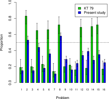
| Figure 1: Proportion of ”A”-answers for the 16 problems in Kahneman and
Tversky (1979) and the present study. Proportions above .50 means that
the modal response was “A”; below means that the modal response was
“B”. Horizontal bars illustrate 95% credible intervals. |
3.3 Choice proportions and modal responses
In Table 2 we see that, as in Kahneman and Tversky (1979), for most
problems there is clear evidence against the null-hypothesis that the
population proportion is .5 (BF10 > 1000:
the exceptions are Problems 2, 4, 8) and for most paradoxes there is
evidence against the choice proportions in the two problems compared
being the same. However, it is only for 11 of the 16 problems that we
replicate the modal response in Kahneman and Tversky. Among these 11
problems, the evidence actually favors H0 (a population
proportion of .5) over H1 for Problem 2 (choice
proportion .530; BF10 = .129) and the evidence for
H1 is weak for Problem 8 (choice proportion .576;
BF10 = 8.85). For the cases where the modal response in
the attempted replication deviates from the original study, the
evidence is very strong (Problems 4, 6, 12, 14, & 15).
As a consequence, in terms of the nine paradoxes, in Kahneman and
Tversky (1979) reported in terms of conflicting modal choices, it is
only for two out of the nine paradoxes (the Certainty Effects with .001
probabilities and the Probabilistic Insurance Effect) that we
unambiguously replicate the modal pattern (e.g., “B” for Problem 1 and
“A’” for Problem 2). As illustrated in Figure 1, there appear to be
systematic differences between our results and those reported by
Kahneman and Tversky, with much more “B” choices in our data. “B” choices
all involve choice of a certain outcome (and are therefore risk averse)
except for Problems 7, 8, 13, and 14, three of which were exceptions to
strong preference for B relative to Kahneman and Tversky.
3.4 Paradoxes at the individual level
Examining the proportion of individuals in the WSD that showed 0, 1,… up
to all 9 paradoxes in Kahneman and Tversky (1979) (i.e., either producing a
EUT-violating AB’ or BA’ choice patterns for the pair of problems), it is
clear that not a single participant (N = 346) produced all nine
paradoxes, the modal participant produced 2 of the 9 paradoxes, and the
median participant produced 3 paradoxes, suggesting that more than 50 % of
the participants exhibited no more than 3 of the 9 original paradoxes (the
patterns of replicated paradoxes are discussed in greater detail in the
next section on the effects of numeracy, and they are summarized in
Appendix B).
3.5 Dependence on Numeracy
3.5.1 Choice proportions and modal responses
Tables C1 to C5 in Appendix C report results for each numeracy group (zero
to four items correct on the BNT) in the same fashion as in Table 2. We
generally replicate the finding that the choice proportions
differ. However, as summarized in Figure 2 (see also Table B1 in Appendix
B), there are notable differences regarding the modal patterns across
numeracy groups. First, the number of modal-pattern replications increase
systematically as the numeracy increases (Table 3). Second, the increases in
modal-pattern replications are related to the paradoxes driven by the
probability weighting function. Third, for the “paradoxes” linked to the
value and the loss function the modal pattern was EUT-consistent choices,
if only because subjects were generally risk averse. When the modal patterns
were not replicated, it was generally not because data yielded insufficient
evidence, but rather because they favored other patterns than in the
original study (e.g., “B” and “B” instead of “B” and “A”). In sum, the modal
results in Kahneman and Tversky (1979) are not replicated for all numeracy
levels and best replicated for the probability-weighting paradoxes and the
most numerate participants.
| Table 3: Replication of the modal response patterns dependent on the
number of items correct on the BNT. “R” illustrate that the statistical
evidence was in favor of replication, minus-sign (“-“) illustrate that
the statistical evidence was in favor of another modal pattern (e.g.,
“B” and “B” instead of “B” and “A”), and “r” illustrate that the
evidence could not decide between the two possibilities. |
| Paradox | Items correct on the BNT |
| | 0 | 1 | 2 | 3 | 4 |
| Certainty effect 1 | - | R | R | R | R |
| Certainty effect 2 | - | r | r | R | R |
| Certainty effect 3 | - | - | r | - | R |
| Certainty effect 4 | - | R | R | R | R |
| Probabilistic insurance | R | R | R | R | R |
| Isolation effect (probabilities) | - | - | - | - | R |
| Isolation effect (outcomes) | - | - | - | - | - |
| Reflection effect for outcomes | - | - | - | - | - |
| Reflection effect (outcomes) | - | - | - | - | - |
| N: | 685 | 508 | 280 | 123 | 37 |
| Table 4: Summary of the patterns of replication of the nine paradoxes in
Kahneman and Tversky (1979) at the level of the individual participant
as a function of numeracy (0 to 4 correct answers on the BNT), together
with indication of the main explanation postulated by Prospect Theory,
either in terms of the value function (VF) or the probability weighting
function (PW). The percentage entries in the table is the percentage of
participants in each category for which the paradox was replicated. For
ease of identification, those categories where the majority of
participants exhibited the paradox are denoted with an asterisk (*). |
| | Explanation | Items correct on the BNT | |
| Paradoxes | VF | PW | 0 | 1 | 2 | 3 | 4 | All |
| Certainty effect 1 | | X | 39% | 44% | 48% | 56% | 75%* | 45% |
| Certainty effect 2 | | X | 27% | 41% | 44% | 44% | 75%* | 38% |
| Certainty effect 3 | | X | 22% | 20% | 37% | 32% | 63%* | 27% |
| Certainty effect 4 | | X | 42% | 57%* | 52%* | 65%* | 88%* | 51%* |
| Probabilistic insurance | | X | 69%* | 74%* | 84%* | 71%* | 63%* | 74%* |
| Isolation effect for probabilities | | X | 28% | 44% | 40% | 41% | 75%* | 38% |
| Isolation effect for outcomes | X | | 22% | 35% | 16% | 32% | 0% | 25% |
| Reflection effect for outcomes | X | | 13% | 16% | 15% | 24% | 25% | 16% |
| Reflection effect for probabilities | X | | 25% | 30% | 33% | 35% | 25% | 29% |
| Average proportion of revealed paradoxes | 32% | 40% | 41% | 44% | 54%* | 38% |
| Average proportion for PW | 38% | 47% | 51%* | 52%* | 73%* | 46% |
| Average proportion for VF | 20% | 27% | 21% | 30% | 17% | 23% |
| Samples sizes N | 130 | 99 | 75 | 24 | 8 | 346 |
3.5.2 Paradoxes at the individual level
A Bayesian ANOVA with number of paradoxes as dependent variable and
numeracy group as the independent variable (parametric assumptions were
satisfied) yielded a BF10 of 52.6 (strong evidence) in
favor of a difference between the numeracy groups (p
< .05; see also Appendix D).
The descriptive statistics summarized in Table 4 strongly suggest that
the observed difference between the numeracy groups is limited to
the paradoxes associated with the probability weighting function. Among
the paradoxes linked to the probability weighting, the EUT-inconsistent
choice pattern was the modal pattern for Numeracy Groups 3, 4, and 5
(for 51%, 52%, and 74% of the participants in each group,
respectively). For “paradoxes” linked to the value function, the
paradoxical choice pattern in Kahneman and Tversky (1979) was never the
most typical pattern (on average observed in 23% of the participants).
Supporting these notions, tests of linear trends using
logistic-regression analysis for each paradox with prevalence of
paradox (yes/no) as the dependent variable and BNT-score as an
independent variable (coded on an interval level) showed significant
effects for Certainty effect 1–4 and the Isolation effect for
probabilities.10
Importantly, the pattern at the level of the individuals (Table 4) is
very similar to the pattern observed for the modal response proportions
(Figure 2). The prevalence of paradoxes is dependent on numeracy.
Figure 2 (Table B2 in Appendix B) show that (i) BB’ was the
most prevalent choice pattern, with increasing frequency as numeracy
decreases; (ii) BA’ choices (which were the choice pattern
emphasized by Kahneman & Tversky, 1979) were the second-most prevalent
pattern with increasing frequency as numeracy increases;
(iii) AA’ responses was the most rare pattern, and with no
visible difference between the numeracy groups; (iv) AB’
responses were the second-most rare pattern, also with no visible
difference between the numeracy groups. This finding is worth
stressing: the difference in the responses is due to how the
participants respond to BB’ or BA’. Notably, B’ as compared to A’, are
options that minimize the risk of obtaining the worst possible outcome,
corresponding to the notion that the less numerate rely on heuristics
that favor less risky options (Cokely & Kelley, 2009), while the more
numerate integrate more of the quantitative information (Reyna et al.,
2014).
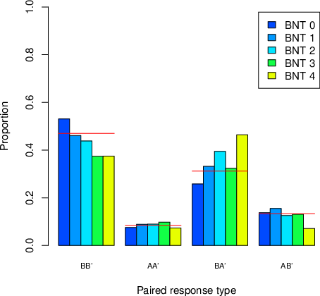
| Figure 2: The proportion of paired responses (y-axis), for each numeracy
group and for all participants (lines), for each paired response type
(x-axis). |
3.5.3 Adressing data quality and noise as a confounding variable
A concern may be that the data for the less numerate participants may be of
lower quality because they, for example, are less motivated to engage in
numerical choice tasks (e.g., Peer, Samat, Brandimart & Acquisti,
2016). Several lines of evidence speak against this interpretation. First,
BNT is seemingly not correlated with measures of motivation (Cokely et al.,
2012). Second, the responses for the least numerate deviate systematically
from .5 and do not seem random or arbitrary. For example, inspecting the
choice proportions for each of the 16 choice problems for the least
numerate (Table B1 in Appendix B), we see that the evidence for a choice
proportion different from .5, over the .5 null-hypothesis of decision
proportion .5 (i.e., random choice), is supported by a BF10
> 1000 for 13 of the 16 problems. The same conclusion is
suggested by the consistent choice pattern by the least numerate in Figure
4, which deviates most distinctly from the uniform distribution expected by
chance responses. The low replication rate at low numeracy is not a result
of more random responses.
Third, there was no evidence that the response times differed between
the BNT groups: a Bayesian ANOVA, with the lognormal-transformed
average response times per prospect as the dependent variable, and BNT
group as the independent variable, yielded a BF10 of
.072 (p>.05); and for the response times for the
BNT test the ANOVA yielded a BF10 of .122
(p>.05).11 It thus
seems unlikely that the less numerate simply wanted to get through the
experiment as quickly as possible and collect their payment. It should
also be noted that our sample also replicated the same positive skew of
responses on the BNT that previous research has documented for similar
crowd source-recruited participants (Cokely et al., 2012); thus, there
was seemingly nothing peculiar with our participants compared to other
similar data samples.
Fourth, assuming that the probability weighting and value functions can
be used to model peoples’ behavior, less reliable responses (i.e., more
“noisy” responses”) should lead to more of the patterns
observed by Kahneman and Tversky (1979), not less: That random noise
contributes to a more nonlinear probability weighting function (and
thus should produce more paradoxes) has been demonstrated elsewhere
(Blavatsky, 2007; Millroth et al., 2018).
A more serious potential problem motivated an independent replication of
our results. Following how we (wrongly) interpreted that Kahneman and
Tversky (1979) conducted their study, we did not counter-balance the
presentation order of the alternatives (i.e., the prospects for
Alternative A, the first choice option, was the same for all
participants). Hypothetically, some of the results reported in Table 2
could be driven by a large proportion of participants having chosen
Alternative B because it was always presented on the right-hand side of
the screen. We therefore conducted an independent replication of the
results in Table 2, where half of the participants received the options
in the same order as in Table 2 (N = 99) and the other half
received the items in the reverse order (N = 100; see Table 4
for results).
In contrast to the hypothesis of a response bias towards Option B (e.g.,
because it is on the right on the computer screen), the response
proportions in Table E1 in Appendix E are mirror images of each other
when the choice options are reversed (i.e., if alternative A was
majority response in the original order, Alternative B was majority
response in the reverse order). The BFDiff in favor of
a difference in the proportions between the two order conditions in
Table 4 were low and ranged between .177 and .466 over the 16 problems
(and between .261 and 1.66, if we only consider the participants with
the lowest numeracy, BNT = 0). Thus, regardless of the presentation of
the choice options, the results in Table E1 replicate the results in
Table 2, but here three out of the nine modal patterns in Kahneman and
Tversky (1979) reappear.12
The consistent mirror effect of reversing the order of the decision
options in Table E1 provides further evidence that the responses
collected here – and by implication the relatively modest replication
rate – are not explained by the participants providing random
responses.
A Bayesian between-subjects ANOVA provides evidence (a
BF10 = 34.3, p <.05) for a
difference in the number of paradoxes between the numeracy groups, with
most replicated paradoxes for participants with highest numeracy (M =
4.75, SD = 2.06) and the lowest number of replicated paradoxes
for participants with lowest numeracy (M = 2.43, SD = 1.52).
In these data, no participant (N = 199) exhibited all 9
paradoxes in the original study.
4 Discussion
The aim of this study was to provide a conceptual replication of the
psychological effects that were reported in the classical study of
Kahneman and Tversky (1979), relating the results to the numeracy of
the participants and the role of contextual support in terms of other
related judgments (raised in terms of the comparison between a WSD and
an SSD). These psychological effects – or decision paradoxes – have in
turn been used to motivate a number of psychological assumptions of PT,
essentially nonlinear probability weighting, nonlinear value functions
that are differently shaped for gains and losses, and an stronger
reaction to losses than to gains of the same magnitude (i.e., loss
aversion). Because we found no strong evidence for systematic
differences in the choice proportions depending on the design type, the
subsequent discussion is focused on the observed differences between
the present study and Kahneman and Tversky (1979) and on how the
results are related to numeracy.
4.1 Replication of the paradoxes in Kahneman and Tversky (1979)
While we replicate that the choice proportions often differ between the two
choice-problems that define a paradox, the results show that for the entire
participant sample the modal responses were clearly replicated only for two
of the nine paradoxes (one Certainty Effect and Probabilistic
Insurance). The conflicting modal choices in these paradoxes were in focus
in Kahneman and Tversky (1979), because they suggested that a majority of
the individuals produced choices that are incompatible with EUT. In our
results, this seems to be most evident for the paradoxes that are related
to the probability weighting function and among the most numerate
participants.13 14 The paradoxes associated with the value function and
loss aversion were harder to replicate in our study. Not a single
individual exhibited all 9 paradoxes posited by PT, and over 50 percent of
all participants exhibited no more than three of the paradoxes. These
conclusions tie into at least two lines of previous research.
First, the prevalence of the reflection effects has indeed varied across
studies (e.g., Ert & Erev, 2013; Harbaugh et al., 2009; Nilsson,
Rieskamp & Wagenmakers, 2011; Yechiam & Hochmann, 2013). The same is
true also for the Isolation Effect for Outcomes (Romanus & Gärling,
1999) and even the Certainty Effect has been shown to depend on the
presentation format (Carlin, 1990; Harbaugh et al., 2009) and the
participant population (Linde & Vis, 2017; Huck & Müller, 2012).
Tellingly, the studies that have most consistently replicated the
original results (Erev et al., 2017; Kühberger et al., 1999) have used
participants recruited from universities; participant that are likely
to exhibit high scores on numeracy.
Second, concerns related to ‘generalized agent models’ (Kirman, 1992)
deserve more attention. For a number of reasons, Kahneman and Tversky
(1979), along with later studies focusing on choice proportions at the
aggregate level, may have over-stated the case for the degree to which
the individual participants disclose the choice patterns that
correspond to the nine paradoxes. Kirman (1992) argued that i)
there may simply be no direct relation between individual and
collective behavior, ii) the generalized agent need not react
to a manipulation in the same manner as the underlying individuals, and
iii), the beliefs by the generalized agent may not be shared
by any of the individuals, but emerges due to the effects of
dispersion. Recent research has shown by simulations that this may hold
for the psychological assumptions of PT (e.g., Jouini & Napp, 2012;
Regenwetter & Robinson, 2017).
The point is not to argue that PT is poorer than EUT as a quantitative
account of the data. By contrast, because PT is more flexible with free
parameters (with EUT as special case) it will trivially be better at
accounting for various patterns observed in data, including those
observed here and those implied by EUT. The ability of a model to
capture also various more idiosyncratic patterns present in a minority
of the participants can be regarded as a virtue of a quantitative
model. Therefore, PT may in many applied circumstances be a more valid
and versatile instrument to describe a variety of different choice
patterns than EUT.
However, the results presented here do raise questions about how
universal the assumptions postulated by PT are and highlight the
importance of determining their limiting conditions. The results in
Kahneman and Tversky (1979) served to motivate and illustrate the key
assumptions of PT, which were intended – as far as we can tell – to
capture important and general aspects of human decision making that
deviate from the assumptions of EUT. It is thus hard to regard the
limited replicability of these phenomena in a wider population as
anything but potentially problematic. As noted above, relaxing EUT in
ways that take psychological assumptions into account can be useful to
capture choice behaviors. The results presented here, however, raise
the question of whether the assumptions made in PT are the most
relevant ones for capturing prevalent deviations from EUT. Moreover,
the application of PT to explain many large-scale societal phenomena
that apparently represent deviations from EUT often seems to presume
that the weighting functions of PT are operative in many or most of the
individual agents. The validity of these assumptions and their
associated effects may also be dependent on the individual
characteristics of the agent, such as his or her level of numeracy. Our
results also question if the account of these paradoxes should be
obligatory benchmarks that any theory of risky decision making in the
field should meet.
4.2 Dependence on numeracy
As noted in the Introduction, the previous literature on numeracy suggested
two contrasting possibilities regarding the outcome of the present
study. The first possibility was that the less numerate would exhibit more
paradoxes because they have a probability-weighting function that is more
nonlinear than the more numerate (Millroth & Juslin, 2015; Patalano et
al., 2015; Schley & Peters, 2014; Traczyk & Fulawka, 2016), and in the
current context a more nonlinear probability weighting function will render
more paradoxes. However, a second possibility pointed to the notion that
the larger observed nonlinearity of the probability weighting function for
lower numeracy has been observed for evaluations of prospects. When people
make choices between prospects, however, the less numerate have been found
to rely on simple heuristics that often favor less risky options (Cokely &
Kelley, 2009), while the numerate are capable of more deliberate behavior,
taking the quantitative details of the problems into account (Cokely &
Kelley, 2009; Reyna et al., 2014).
The results showed that the least numerate exhibited the fewest
paradoxes at the individual level, and the most numerate exhibited most
paradoxes at the individual level. The differences was constrained to
the paradoxes that relate to the probability weighting function
proposed by Kahneman and Tversky (1979; see also Tversky and Kahneman,
1992). Most of the effects of numeracy were consistent with a
systematic shift in the less numerate to a more cautious
non-compensatory strategy that minimized the risk of obtaining the
worst possible outcome, in line with the second possibility. The simple
strategy of rejecting the option with the poorest possible outcome or,
if all options have this same poorest outcome as a possibility, to
reject the option with the higher probability of this poor outcome,
predicts Option B for all choice problems in Table 1, which corresponds
to the decision behavior at low numeracy (see Table C1 in Appendix C).
Researchers therefore need to be aware of the implications: the
preferences captured in any given experiment is likely to depend on an
interaction between the type of elicitation method (evaluations vs.
choices) and level of numeracy. This is in line with a growing body of
research that has documented the malleability of preferences derived
from behavioral measures (e.g., Pedroni et al., 2017): rather than
having stable risk preferences that can be fundamentally different
between people, it seems that people are instead probably equipped with
a large variety of decision strategies that they apply in response to
the specific architecture of the environment.
We found no evidence that these patterns were explained by “random
responses” or poor data quality. The responses provided at low numeracy
seem highly systematic and when the order of the choice options are
reversed, so are the choice between the alternatives (i.e., if the
participants choose Option A in the original order they seem to select
Option B when the options are presented in the reverse order). Neither
were there differences in the response times to the prospects, nor to
the BNT. Future research could usefully include other measures of
numeracy (e.g., the Lipkus-test), measures of motivation and of
metacognition, in order to elucidate the exact mechanisms by which the
differences numeracy causes the result.
4.3 Why is numeracy positively related to the susceptibility to
(some) paradoxes?
In the following, we entertain two (not necessarily exclusive)
explanations. A first explanation emphasizes that the kind of
lottery-metaphor tasks typically used in decision research (and in this
study) may be cognitively more demanding to people with low numeracy.
People low in numeracy may therefore find it especially difficult to
confidently evaluate these complex quantitative options and instead
they may retreat to the more cautious strategy of minimizing the risk
of receiving the worst possible outcome, the pattern observed in our
data.
On the one hand, this attitude makes some sense (i.e., even those high
in numeracy could presumably be presented with lottery options that are
so complex that they are difficult to evaluate, which they therefore
are inclined to reject ) and in regard to the specific choice set in
Kahneman and Tversky (1979) it leads to better agreement with EUT. On
the other hand, and in the large scheme of things, inability to
properly integrate probabilities and outcomes to identify superior
options will often produce mediocre decisions with poorer long-term
accrual of returns. This can be considered as an epistemic risk
aversion, where people avoid not only the options where the outcome
obtained is unknown, but also the options for which they lack
sufficient confidence in their own ability to accurately evaluate their
attractiveness. Future research should delineate to what extent this
holds under varying conditions (i.e., numerically simplifying things in
terms of attributes and alternatives),
A second potential explanation is provided by fuzzy-trace theory (FTT:
Brainers & Reyna, 1990; Reyna & Brainerd, 1995; Reyna, 2008; Reyna &
Brainerd, 2011; Broniatowski & Reyna, 2018). FTT posits that people rely
on two types of mental representations: verbatim and gist
representations. Verbatim representations capture the exact surface form of
problems or situations, how they are perceived literally (e.g., the words
or numbers). Gist captures the bottom-line meaning of the problem or
situation. In contrast to verbatim representations, which are precise (and
quantitative, if they involve numbers), gist representations are vague and
qualitative. People are capable of processing both verbatim and gist
information, but they prefer to reason with gist traces rather than
verbatim. Importantly, FTT can explain the functional forms of probability
and value posited by PT (for the mathematics, see Reyna & Brainerd, 2011;
Broniatowski & Reyna, 2018). A hypothesis in the framework of FFT is that,
in choices between risky prospects, the least numerate rely on
gist-representations while the more numerate are more able to make use of
verbatim quantitative representations.
4.4 Conclusions
We believe that our study demonstrates that i) the replication
rate for the paradoxes in Kahneman and Tversky(1979) that originally
motivated the key psychological assumptions of PT is very modest in a
population with a larger variation in numeracy; ii) The
paradoxes that are easiest to replicate are those that relate to the
probability weighting function, but they primarily occur among
participants that are high numeracy; and iii) The choices in
people low in numeracy make are consistent with a shift towards a more
cautious and non-compensatory strategy that concentrates on minimizing
the risk of obtaining the worst outcome. The results highlight
important limiting conditions for the psychological assumptions made in
PT.
References
Birnbaum, M. H. (1999). Paradoxes of Allais, stochastic dominance, and
decision weights. Decision science and technology: Reflections
on the contributions of Ward Edwards, 27–52.
Birnbaum, M. H. (2008). New paradoxes of risky decision
making. Psychological Review, 115(2), 463–501.
Reyna, V. F., & Brainerd, C. J. (1995). Fuzzy-trace theory: Some
foundational issues. Learning and Individual
differences, 7(2), 145–162.
Brandstätter, E., Gigerenzer, G., & Hertwig, R. (2006). The priority
heuristic: making choices without trade-offs. Psychological
Review, 113(2), 409–432.
Broniatowski, D. A., & Reyna, V. F. (2018). A Formal Model of
Fuzzy-Trace Theory: Variations on Framing Effects and the Allais
Paradox. Decision, 5(4), 205–252.
Camerer, C. F., Dreber, A., Forsell, E., Ho, T. H., Huber, J.,
Johannesson, M., ... & Heikensten, E. (2016). Evaluating replicability
of laboratory experiments in
economics. Science, 351(6280), 1433–1436.
Camerer, C., Babcock, L., Loewenstein, G., & Thaler, R. (1997). Labor
supply of New York City cabdrivers: One day at a time. The
Quarterly Journal of Economics, 112(2), 407–441.
Carlin, P. S. (1990). Is the Allais paradox robust to a seemingly
trivial change of frame?. Economics Letters, 34(3),
241–244.
Cokely, E. T., & Kelley, C. M. (2009). Cognitive abilities and superior
decision making under risk: A protocol analysis and process model
evaluation. Judgment and Decision Making, 4(1), 20–33.
Cokely, E. T., Feltz, A., Ghazal, S., Allan, J. N., Petrova, D., & Garcia-Retamero, R. (2017). Decision making skill:
From intelligence to numeracy and expertise. Cambridge Handbook of
Expertise and Expert Performance, 2nd, Cambridge University Press, New
York NY.
Cokely, E. T., Galesic, M., Schulz, E., Ghazal, S., & Garcia-Retamero,
R. (2012). Measuring risk literacy: The Berlin numeracy
test. Judgment and Decision Making, 7(1), 25–47.
Dienes, Z. (2014). Using Bayes to get the most out of non-significant
results. Frontiers in Psychology, 5, Article ID 781.
Erev, I., Ert, E., Plonsky, O., Cohen, D., & Cohen, O. (2017). From
anomalies to forecasts: Toward a descriptive model of decisions under
risk, under ambiguity, and from experience. Psychological
Review, 124(4), 369–409.
Erev, I., & Wallsten, T. S. (1993). The effect of explicit
probabilities on decision weights and on the reflection
effect. Journal of Behavioral Decision Making, 6(4), 221–241.
Fennema, H., & Wakker, P. (1997). Original and cumulative prospect
theory: A discussion of empirical differences. Journal of
Behavioral Decision Making, 10(1), 53–64.
Fleming, S. M., Maloney, L. T., & Daw, N. D. (2013). The irrationality
of categorical perception. Journal of Neuroscience, 33(49),
19060–19070.
Fox, C. R., & Poldrack, R. A. (2009). Prospect theory and the brain.
In Glimcher, P.W., & Fehr, E. (Eds). Neuroeconomics: Decision
making and the brain (pp. 145–173). Academic Press. New York.
Ghazal, S., Cokely, E. T., & Garcia-Retamero, R. (2014). Predicting
biases in very highly educated samples: Numeracy and
metacognition. Judgment and Decision Making, 9(1), 15–34.
Gigerenzer, G. (2017). A theory integration
program. Decision, 4(3), 133–145.
Gosling, S. D., & Mason, W. (2015). Internet research in
psychology. Annual Review of Psychology, 66, 877–902.
Grawitch, M. J., & Munz, D. C. (2004). Are your data nonindependent? A
practical guide to evaluating nonindependence and within-group
agreement. Understanding Statistics, 3(4), 231–257.
Harbaugh, W. T., Krause, K., & Vesterlund, L. (2010). The fourfold
pattern of risk attitudes in choice and pricing tasks. The
Economic Journal, 120(545), 595–611.
Hauser, D. J., & Schwarz, N. (2016). Attentive Turkers: MTurk
participants perform better on online attention checks than do subject
pool participants. Behavior Research Methods, 48(1), 400–407.
Huck, S., & Müller, W. (2012). Allais for all: Revisiting the paradox
in a large representative sample. Journal of Risk and
Uncertainty, 44(3), 261–293.
Jervis, R. (1992). Political implications of loss
aversion. Political Psychology, 187–204.
Jouini, E., & Napp, C. (2012). Behavioral biases and the representative
agent. Theory and Decision, 73(1), 97–123.
Kahneman, D., & Tversky, A. (1979). Prospect Theory: An Analysis of
Decision under Risk. Econometrica, 47(2), 263–292.
Kahneman, D., & Frederick, S. (2005). A model of heuristic
judgment. The Cambridge handbook of thinking and reasoning,
267–293.
Kirman, A. P. (1992). Whom or what does the representative individual
represent?. The Journal of Economic Perspectives, 6(2),
117–136.
Kühberger, A., Schulte-Mecklenbeck, M., & Perner, J. (1999). The
effects of framing, reflection, probability, and payoff on risk
preference in choice tasks. Organizational Behavior and Human
Decision Processes, 78(3), 204–231.
Levy, J. S. (1996). Loss aversion, framing, and bargaining: The
implications of prospect theory for international
conflict. International Political Science Review, 17(2),
179–195.
Lichtenstein, S., & Slovic, P. (Eds.). (2006). The construction
of preference. Cambridge University Press.
Lilienfeld, S. O., & Waldman, I. D. (Eds.).
(2017). Psychological science under scrutiny: Recent challenges
and proposed solutions. John Wiley & Sons.
Linde, J., & Vis, B. (2017). Do politicians take risks like the rest of
us? An experimental test of prospect theory under
MPs. Political Psychology, 38(1), 101–117.
Lindskog, M., Kerimi, N., Winman, A., & Juslin, P. (2015). A Swedish
validation of the Berlin numeracy test. Scandinavian Journal of
Psychology, 56(2), 132–139.
Lipkus, I. M., Samsa, G., & Rimer, B. K. (2001). General performance on
a numeracy scale among highly educated samples. Medical
Decision Making, 21(1), 37–44.
Låg, T., Bauger, L., Lindberg, M., & Friborg, O. (2014). The role of
numeracy and intelligence in health-risk estimation and medical data
interpretation. Journal of Behavioral Decision Making, 27(2),
95–108.
Mallpress, D. E., Fawcett, T. W., Houston, A. I., & McNamara, J. M.
(2015). Risk attitudes in a changing environment: An evolutionary model
of the fourfold pattern of risk preferences. Psychological
Review, 122(2), 364–375.
McDermott, R., Fowler, J. H., & Smirnov, O. (2008). On the evolutionary
origin of prospect theory preferences. The Journal of
Politics, 70(2), 335–350.
Millroth, P., & Juslin, P. (2015). Prospect evaluation as a function of
numeracy and probability denominator. Cognition, 138, 1–9.
Millroth, P., Nilsson, H., & Juslin, P. (2018). Examining the integrity
of evaluations of risky prospects using a single-stimuli design.
Decision, 5(4), 362–377.
Morey, R. D., Rouder, J. N., & Jamil, T. (2015). BayesFactor:
Computation of Bayes factors for common designs. R package version
0.9, 9.
Morey, R. D., & Rouder, J. N. (2011). Bayes factor approaches for
testing interval null hypotheses. Psychological
Methods, 16(4), 406–419.
Mukherjee, S., Sahay, A., Pammi, V. C., & Srinivasan, N. (2017). Is
loss-aversion magnitude-dependent? Measuring prospective affective
judgments regarding gains and losses. Judgment and Decision
Making, 12(1), 81–89.
Nilsson, H., Rieskamp, J., & Wagenmakers, E. J. (2011). Hierarchical
Bayesian parameter estimation for cumulative prospect
theory. Journal of Mathematical Psychology, 55(1), 84–93.
Obrecht, N. A., Chapman, G. B., & Gelman, R. (2009). An encounter
frequency account of how experience affects likelihood
estimation. Memory & Cognition, 37(5), 632–643.
Open Science Collaboration. (2015). Estimating the reproducibility of
psychological science. Science, 349(6251), aac4716.
Pachur, T., & Galesic, M. (2013). Strategy selection in risky choice:
The impact of numeracy, affect, and cross-cultural
differences. Journal of Behavioral Decision Making, 26(3),
260–271.
Patalano, A. L., Saltiel, J. R., Machlin, L., & Barth, H. (2015). The
role of numeracy and approximate number system acuity in predicting
value and probability distortion. Psychonomic Bulletin & Review, 22(6), 1820–1829.
Pedroni, A., Frey, R., Bruhin, A., Dutilh, G., Hertwig, R., & Rieskamp,
J. (2017). The risk elicitation puzzle. Nature Human
Behaviour, 1(11), 803–809.
Peer, E., Samat, S., Brandimarte, L., & Acquisti, A. (2016). Beyond the
Turk: An empirical comparison of alternative platforms for
crowdsourcing online behavioral research.
https://www.ssrn.com/abstract=2594183
Peters, E., Baker, D. P., Dieckmann, N. F., Leon, J., & Collins, J.
(2010). Explaining the effect of education on health: A field study in
Ghana. Psychological Science, 21(10), 1369–1376.
Peters, E., & Bjalkebring, P. (2015). Multiple numeric competencies:
When a number is not just a number. Journal of
Personality and Social Psychology, 108(5), 802–822.
Peters, E., Västfjäll, D., Slovic, P., Mertz, C. K., Mazzocco, K., &
Dickert, S. (2006). Numeracy and decision making. Psychological
Science, 17(5), 407–413.
Regenwetter, M., Dana, J., & Davis-Stober, C. P. (2011). Transitivity
of preferences. Psychological Review, 118(1), 42–56.
Regenwetter, M., Grofman, B., Popova, A., Messner, W., Davis-Stober, C.
P., & Cavagnaro, D. R. (2009). Behavioural social choice: a status
report. Philosophical Transactions of the Royal Society of
London B: Biological Sciences, 364(1518), 833–843.
Regenwetter, M., & Robinson, M. M. (2017). The construct–behavior gap
in behavioral decision research: A challenge beyond
replicability. Psychological Review, 124(5), 533–550.
Reyna, V. F. (2008). A theory of medical decision making and health:
fuzzy trace theory. Medical Decision Making, 28(6), 850–865.
Reyna, V. F., & Brainerd, C. J. (1995). Fuzzy-trace theory: An interim
synthesis. Learning and Individual Differences, 7(1), 1–75.
Reyna, V. F., & Brainerd, C. J. (2011). Dual processes in decision
making and developmental neuroscience: A fuzzy-trace
model. Developmental Review, 31(2), 180–206.
Reyna, V. F., & Brainerd, C. J. (2008). Numeracy, ratio bias, and
denominator neglect in judgments of risk and
probability. Learning and Individual Differences, 18(1),
89–107.
Reyna, V. F., Chick, C. F., Corbin, J. C., & Hsia, A. N. (2014).
Developmental reversals in risky decision making: Intelligence agents
show larger decision biases than college
students. Psychological Science, 25(1), 76–84.
Reyna, V. F., Nelson, W. L., Han, P. K., & Dieckmann, N. F. (2009). How
numeracy influences risk comprehension and medical decision
making. Psychological Bulletin, 135(6), 943–973.
Romanus, J., & Gärling, T. (1999). Do changes in decision weights
account for effects of prior outcomes on risky decisions?. Acta
Psychologica, 101(1), 69–78.
Rouder, J. N., Speckman, P. L., Sun, D., Morey, R. D., & Iverson, G.
(2009). Bayesian t tests for accepting and rejecting the null
hypothesis. Psychonomic Bulletin & Review, 16(2), 225–237.
Schley, D. R., & Peters, E. (2014). Assessing “economic value”
symbolic-number mappings predict risky and riskless
valuations. Psychological Science, 25(3), 753–761.
Schwartz, L. M., Woloshin, S., Black, W. C., & Welch, H. G. (1997). The
role of numeracy in understanding the benefit of screening
mammography. Annals of Internal Medicine, 127(11), 966–972.
Segal, U. (1988). Probabilistic insurance and anticipated
utility. Journal of Risk and Insurance, 287–297.
Shaffer, J. P. (1972). Directional statistical hypotheses and
comparisons among means. Psychological Bulletin, 77(3), 195–197.
Smith, E. R., & Semin, G. R. (2007). Situated social
cognition. Current Directions in Psychological Science, 16(3),
132–135.
Traczyk, J., & Fulawka, K. (2016). Numeracy moderates the influence of
task-irrelevant affect on probability
weighting. Cognition, 151, 37–41.
Tversky, A., & Kahneman, D. (1992). Advances in prospect theory:
Cumulative representation of uncertainty. Journal of Risk and
Uncertainty, 5(4), 297–323.
Wagenmakers, E. J. (2007). A practical solution to the pervasive
problems of p values. Psychonomic Bulletin & Review, 14(5),
779–804.
Wakker, P., Thaler, R., & Tversky, A. (1997). Probabilistic
insurance. Journal of Risk and Uncertainty, 15(1), 7–28.
Winman, A., Juslin, P., Lindskog, M., Nilsson, H., & Kerimi, N. (2014).
The role of ANS acuity and numeracy for the calibration and the
coherence of subjective probability judgments. Frontiers in
Psychology, 5, Article ID 851.
Yechiam, E., & Hochman, G. (2013). Losses as modulators of attention:
review and analysis of the unique effects of losses over
gains. Psychological Bulletin, 139(2), 497–518.
Yeh, W., & Barsalou, L. W. (2006). The situated nature of
concepts. The American Journal of Psychology, 349–384.
Zynda, L. (1996). Coherence as an ideal of
rationality. Synthese, 109(2), 175–216.
5 Appendix A: Detailed Report of Statistics Related to Design
(WSD or SSD)
To determine whether the modal responses differed between the samples,
proportions along with 95 per cent credible intervals were derived using
Bayesian binomial tests. To quantify the evidence that a proportion was
either mostly “A” or mostly “B” we calculated a Bayes factor (BF) for each
problem that tested the contrasts that the proportion of answer “A” was
below .50 or over .50. This BF is obtained by first computing a Bayesian
binomial test for a positive difference vs. a point null-hypothesis of
zero difference to obtain a first BF and then computing a Bayesian binomial
test for a negative difference vs. a point null-hypothesis of zero
difference to obtain as second BF. The BF directly contrasting a positive
vs. a negative difference is obtained by taking the ratio of the BFs for
the positive and negative difference. The proportion was categorized as A
or B if the BF was over three, as this at least can be considered “positive
evidence” (Kass & Raftery, 1996). The results are summarized in Table A1,
showing that the modal responses were the same for both samples.
Table A1: Proportion of “A” (Yes for item 9) responses for all 16 items
dependent on design (WSD or SSD) along with BFs quantifying the
evidence that proportion is over/under .50. Proportions within
parentheses show lower and upper 95% credible intervals.
| Prob. | WSD proportions | BF | SSD proportions | BF |
| 1 | .133 (.101; .173) | >103 | .239 (.162; .338) | >103 |
| 2 | .523 (470; .575) | 4.13 | .562 (.441; .662) | 4.61 |
| 3 | .153 (.119; .195) | >103 | .145 (.085; .236) | >103 |
| 4 | .457 (.405; .509) | 17.9 | .368 (.269; .481) | 90.6 |
| 5 | .182 (.145; .226) | >103 | .153 (.092; .245) | >103 |
| 6 | .367 (.318; .419) | >103 | .345 (.252; .452) | 439 |
| 7 | .110 (.081; .147) | >103 | .116 (.065; .201) | >103 |
| 8 | .587 (.534; .637) | >103 | .532 (.422; .638) | 2.48* |
| 9 | .263 (.219; .312) | >103 | .387 (.294; .489) | 66 |
| 10 | .159 (.124; .201) | >103 | .186 (.112; 293) | >103 |
| 11 | .202 (.163; .248) | >103 | .400 (.301; .507) | 29.5 |
| 12 | .335 (.288; .387) | >103 | Missing | |
| 13 | .379 (.329; .431) | >103 | .417 (.310; .532) | 11.51 |
| 14 | .263 (.219; .312) | >103 | .368 (.269; .481) | 90.6 |
| 15 | .367 (.318; .419) | >103 | .301 (.213; .407) | >103 |
| 16 | .243 (201; .291) | >103 | .262 (.213; .407) | >103 |
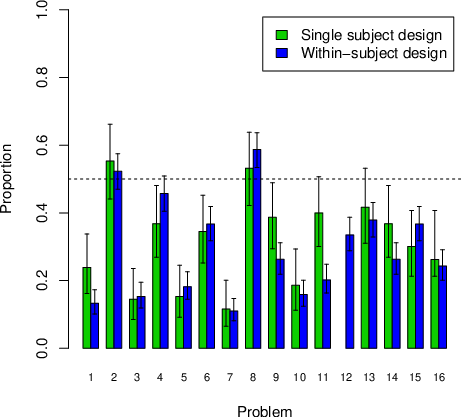
Figure A1: The mean proportions “Decision A” with 95% credible
intervals for the 16 decisions problems summarized in Table 1 observed
in the present experiment, separately for the data from the Single
Subject Design (SSD) and the Within-Subject Design (WSD).
6 Appendix B: Proportion of Paradoxes
Table B1 report the proportion of participants, for each numeracy group
and for all participants, which exhibited a specific number of
paradoxes. Table B2 report the proportion of responses, for each
numeracy group and for all participants, for each observed
paired-response type.
Table B1: The proportion of participants that exhibited a specific
number of paradoxes for each numeracy group and for all participants in
the WSD.
| | Number of Paradoxes |
| Group | 0 | 1 | 2 | 3 | 4 | 5 | 6 | 7 | 8 | 9 |
| O on BNT | .077 | .162 | .238 | .215 | .092 | .115 | .069 | .023 | .008 | .000 |
| 1 on BNT | .020 | .141 | .202 | .141 | .121 | .162 | .131 | .071 | .010 | .000 |
| 2 on BNT | .000 | .213 | .133 | .120 | .147 | .160 | .133 | .080 | .013 | .000 |
| 3 on BNT | .000 | .088 | .147 | .088 | .412 | .059 | .088 | .059 | .059 | .000 |
| 4 on BNT | .000 | .000 | .125 | .125 | .125 | .125 | .375 | .125 | .000 | .000 |
| All participants | .035 | .156 | .194 | .159 | .145 | .133 | .110 | .055 | .014 | .000 |
Table B2: The proportion of responses, for each numeracy group and for
all participants, for each observed paired-response type in the WSD.
| | Paired-Response Type |
| Group | BB’ | AA’ | BA’ | AB’ |
| O on BNT | .534 | .069 | .241 | .156 |
| 1 on BNT | .436 | .096 | .298 | .170 |
| 2 on BNT | .458 | .092 | .290 | .160 |
| 3 on BNT | .371 | .088 | .353 | .188 |
| 4 on BNT | .359 | .078 | .406 | .156 |
| All participants | .469 | .084 | .283 | .164 |
7 Appendix C: Results for Each Numeracy Group
Table C1 to C5 summarize the detailed results for each numeracy group.
Table C1: Proportion of “A” (Yes for Item 9) responses for all 16 items of
the present study for the participants with 0 items correct on the BNT
(parentheses show lower and upper 95% credible Intervals) along with three
Bayes factors (BFs). BF
10 quantifies the evidence against
the proportion being .5. BF
Dir quantifies the evidence in
favor of the proportion being in the observed Direction as opposed to the
other direction. BF
Diff quantifies the evidence against the
choice proportions in the relevant choice problems being the same.
| Effect | Problem | Choice proportion | BF10 against .50 | Majority choice | BFDir | BFDiff |
| Certainty effect | 1 | .166 (.118; .228) | >103 | B | >103 | >103 |
| | 2 | .442 (.369; .519) | 0.289 | B | −13.4 | |
| Certainty effect | 3 | .145 (.099; .208) | >103 | B | >103 | 182 |
| | 4 | .323 (.257; .298) | >103 | B | >103 |
| Certainty effect | 5 | .169 (.122; .232) | >103 | B | >103 | 11.9 |
| | 6 | .309 (.244; .383) | >103 | B | >103 |
| Certainty effect | 7 | .109 (.070; .166) | >103 | B | >103 | >103 |
| | 8 | .472 (.396; .549) | 7.85 | B | 3.18 | |
| Probabilistic insurance | 9 | .323 (.257; .398) | >103 | No | >103 | |
| Isolation effect for Probabilities | 10 | .261 (.199; .334) | >103 | B | >103 | 0.23 |
| Isolation effect for outcomes | 11 | .229 (.172; .299) | >103 | B | >103 | 0.313 |
| | 12 | .300 (.228; .384) | >103 | B | >103 | |
| Reflection effect for outcomes | 13 | .384 (.312; .461) | 0.135 | B | −592 | 0.616 |
| | 14 | .283 (.220; .356) | >103 | B | >103 | |
| Reflection effect for probabilities | 15 | .325 (.259; .399) | >103 | B | >103 | 0.271 |
| | 16 | .256 (.187; .335) | >103 | B | >103 | |
Table C2: Proportion of “A” (Yes for Item 9) responses for all
16 items of the present study for the participants with 1 items correct
on the BNT (parentheses show lower and upper 95% credible Intervals)
along with three Bayes factors (BFs). BF
10 quantifies
the evidence against the proportion being .5. BF
Dir
quantifies the evidence in favor of the proportion being in the
observed Direction as opposed to the other
direction. BF
Diff quantifies the evidence against the
choice proportions in the relevant choice problems being the same.
| Effect | Problem | Choice proportion | BF10 against .50 | Majority
choice | BFDir | BFDiff |
| Certainty effect | 1 | .146 (.095; .220) | >103 | B | >103 | >103 |
| | 2 | .558 (.469; .644) | 0.256 | A | −8.85 | |
| Certainty effect | 3 | .150 (.100; .221) | >103 | B | >103 | >103 |
| | 4 | .512 (.424; .600) | 0.117 | Indifference | −1.55 | |
| Certainty effect | 5 | .192 (.133; .270) | >103 | B | >103 | 2.9 |
| | 6 | .331 (.254; .418) | 149 | B | >103 | |
| Certainty effect | 7 | .118 (.073; .186) | >103 | B | >103 | >103 |
| | 8 | .653 (.564; .732) | 33.9 | A | >103 | |
| Probabilistic insurance | 9 | .274 (.206; .355) | >103 | No | >103 | |
| Isolation effect for Probabilities | 10 | .293 (.220; .379) | >103 | B | >103 | 44.7 |
| Isolation effect for outcomes | 11 | .240 (.174; .322) | >103 | B | >103 | 33.6 |
| | 12 | .455 (.360; .553) | 0.188 | Indifference | −4.43 | |
| Reflection effect for outcomes | 13 | .405 (.322; .494) | 1 | B | −53.2 | 2.08 |
| | 14 | .258 (.188; .344) | >103 | B | >103 | |
| Reflection effect for probabilities | 15 | .402 (.320; .489) | 1.29 | B | −105 | 0.655 |
| | 16 | .287 (.214; .373) | >103 | B | >103 | |
Table C3: Proportion of “A” (Yes for Item 9) responses for all 16 items of
the present study for the participants with 2 items correct on the BNT
(parentheses show lower and upper 95% credible Intervals) along with three
Bayes factors (BFs). BF
10 quantifies the evidence against
the proportion being .5. BF
Dir quantifies the evidence in
favor of the proportion being in the observed Direction as opposed to the
other direction. BF
Diff quantifies the evidence against the
choice proportions in the relevant choice problems being the same.
| Effect | Problem | Choice proportion | BF10 against .50 | Majority
choice | BFDir | BFDiff |
| Certainty effect | 1 | .163 (.100; .255) | >103 | B | >103 | >103 |
| | 2 | .575 (.470; .674) | 0.349 | A | −11 | |
| Certainty effect | 3 | .146 (.086; .239) | >103 | B | >103 | >103 |
| | 4 | .483 (.381; .586) | 0.14 | Indifference | −1.67 | |
| Certainty effect | 5 | .146 (.086; .239) | >103 | B | >103 | >103 |
| | 6 | .473 (.373; .574) | 0.149 | Indifference | −2.32 | |
| Certainty effect | 7 | .108 (.060; .187) | >103 | B | >103 | >103 |
| | 8 | .574 (.473; .670) | 0.361 | A | −12.4 | |
| Probabilistic insurance | 9 | .167 (.102; .261) | >103 | No | >103 | |
| Isolation effect for Probabilities | 10 | .253 (.168; .349) | >103 | B | >103 | 40.1 |
| Isolation effect for outcomes | 11 | .261 (.181; .362) | >103 | B | >103 | 1.64 |
| | 12 | .253 (.169; .363) | >103 | B | >103 | |
| Reflection effect for outcomes | 13 | .386 (.291; .491) | 1.27 | B | −58.4 | 0.416 |
| | 14 | .277 (.192; .382) | 628 | B | >103 | |
| Reflection effect for probabilities | 15 | .337 (.247; .441) | 15.3 | B | 226 | 2.91 |
| | 16 | .176 (.110; .271) | >103 | B | >103 | |
Table C4: Proportion of “A” (Yes for Item 9) responses for all 16 items of
the present study for the participants with 3 items correct on the BNT
(parentheses show lower and upper 95% credible Intervals) along with three
Bayes factors (BFs). BF
10 quantifies the evidence against
the proportion being .5. BF
Dir quantifies the evidence in
favor of the proportion being in the observed Direction as opposed to the
other direction. BF
Diff quantifies the evidence against the
choice proportions in the relevant choice problems being the same.
| Effect | Problem | Choice proportion | BF10 against .50 | Majority
choice | BFDir | BFDiff |
| Certainty effect | 1 | .073 (.027; .195) | >103 | B | >103 | >103 |
| | 2 | .605 (.446; .744) | 0.456 | A | −9.01 | |
| Certainty effect | 3 | .233 (.132; .378) | 104 | B | >103 | 25.7 |
| | 4 | .583 (.421; .729) | 0.334 | A | −5.18 | |
| Certainty effect | 5 | .231 (.127; .385) | 64.9 | B | >103 | 0.381 |
| | 6 | .341 (.216; .495) | 1.49 | B | −44.7 | |
| Certainty effect | 7 | .128 (.057; .268) | >103 | B | >103 | >103 |
| | 8 | .750 (.597; 858) | 31.6 | A | >103 | |
| Probabilistic insurance | 9 | .409 (.277; .557) | 0.38 | No | −7.63 | |
| Isolation effect for Probabilities | 10 | .297 (.175; 459) | 4.23 | B | −142 | 3.23 |
| Isolation effect for outcomes | 11 | .293 (.176; .446) | 6.63 | B | −254 | 2.76 |
| | 12 | .382 (.239; .551) | 0.529 | B | −10.4 | |
| Reflection effect for outcomes | 13 | .357 (.230; .509) | 1.04 | B | −29.5 | 0.213 |
| | 14 | .308 (.186; .465) | 3.51 | B | −120 | |
| Reflection effect for probabilities | 15 | .371 (.239; .551) | 0.646 | B | −14 | 0.331 |
| | 16 | .257 (.146; .433) | 13.5 | B | 333 | |
Table C5: Proportion of “A” (Yes for Item 9) responses for all 16 items of
the present study for the participants with 4 items correct on the BNT
(parentheses show lower and upper 95% credible Intervals) along with three
Bayes factors (BFs). BF
10 quantifies the evidence against
the proportion being .5. BF
Dir quantifies the evidence in
favor of the proportion being in the observed Direction as opposed to the
other direction. BF
Diff quantifies the evidence against the
choice proportions in the relevant choice problems being the same.
| Effect | Problem | Choice proportion | BF10 against .50 | Majority
choice | BFDir | BFDiff |
| Certainty effect | 1 | .333 (.122; .652) | 0.61 | B | −4.81 | 31.6 |
| | 2 | 1.00 (.692; 1.00) | 51.2 | A | >103 | |
| Certainty effect | 3 | .000 (.000; .247) | 315 | B | >103 | 92.9 |
| | 4 | .636 (.349; .848) | 0.517 | A | (>103) | |
| Certainty effect | 5 | .125 (.028; .482) | 3.56 | B | −4.15 | 9.38 |
| | 6 | .778 (.444; .933) | 1.42 | A | −50.2 | |
| Certainty effect | 7 | .000 (.000; .336) | 28.4 | B | >103 | 19.1 |
| | 8 | .636 (.349; .848) | 0.517 | A | −17.2 | |
| Probabilistic insurance | 9 | .444 (.187; .738) | 0.406 | No | −4.15 | |
| Isolation effect for Probabilities | 10 | .200 (.060; .518) | 2.07 | B | −29.6 | 1.98 |
| Isolation effect for outcomes | 11 | .091 (.021; .385) | 15.5 | B | 316 | 0.864 |
| | 12 | .000 (.000; .336) | 28.4 | B | >103 | |
| Reflection effect for outcomes | 13 | .250 (.075; .600) | 1.02 | B | −10.1 | 0.423 |
| | 14 | .429 (.213; .677) | 0.364 | B | −2.29 | |
| Reflection effect for probabilities | 15 | .333 (.122; .652) | 0.61 | B | −4.81 | 0.81 |
| | 16 | .111 (.025; .445) | 5.69 | B | −50.2 | |
8 Appendix D: Post-Hoc Comparisons for ANOVA of Paradoxes at the
Individual Level
While JASP allow for post-hoc testing of the ANOVA, those tests test only
against the null, and arguably directional hypotheses are generally more
desirable (see e.g., Morey & Rouder, 2011; Shaffer, 1972). Thus, we again
used directional hypothesis testing (Morey & Rouder, 2011). The results in
Table D1 show that that the least numerate produce fewer paradoxes than all
other groups, but also that the most numerate exhibit more paradoxes than
the groups that scored one or two items correct on the BNT. The evidence is
even stronger when the paradoxes of Probabilistic Insurance, Isolation
Effect for Outcomes, and the Reflection Effects are excluded from analysis
(a reasonable exclusion, because the groups did not differ in regard to
these paradoxes), as also illustrated in Table D1.
Table D1: Results from contrasting Bayesian t-testing of mean number of
exhibited effects for participants in the WSD (95 per cent credible
intervals in parentheses) for each possible group comparison, both for
when all paradoxes were included in the analysis and when three
Paradoxes that no group exhibited were excluded from the
analysis.
Compared BNT groups | Mean # of exhibited effects | Favored hypothesis
(all) | BF | Favored hypothesis (excluded) | BF |
0 vs. 1 | 2.87 vs. 3.63 (2.55; 3.19) (3.23; 4.02) | 0 < 1 | 512 | 0 < 1 | 79.9 |
0 vs. 2 | 2.87 vs. 3.69 (2.55; 3.19) (3.22; 4.16) | 0 < 2 | 473 | 0 < 2 | 216 |
0 vs. 3 | 2.87 vs. 4.00 (2.55; 3.19) (3.35; 4.65) | 0 < 3 | 746 | 0 < 3 | 187 |
0 vs. 4 | 2.87 vs. 4.88 (2.55; 3.19) (3.43; 6.32) | 0 < 4 | 242 | 0 < 4 | >1,000 |
1 vs. 2 | 3.63 vs. 3.69 (3.23; 4.02) (3.22; 4.16) | 1 < 2 | 1.4 | 1 ≠ 2 | 5.24 |
1 vs. 3 | 3.63 vs. 4.00 (3.23; 4.02) (3.35; 4.65) | 1 < 3 | 4.46 | 1 < 3 | 4.49 |
1 vs. 4 | 3.63 vs. 4.88 (3.23; 4.02) (3.43; 6.32) | 1 < 4 | 13.5 | 1 < 4 | 125 |
2 vs. 3 | 3.69 vs. 4.00 (3.22; 4.16) (3.35; 4.65) | 2 < 3 | 3.12 | 2 ≠ 3 | 4.16 |
2 vs. 4 | 3.69 vs. 4.88 (3.22; 4.16) (3.43; 6.32) | 2 < 4 | 10.24 | 2 < 4 | 49.6 |
3 vs. 4 | 4.00 vs. 4.88 (3.35; 4.65) (3.43; 6.32) | 3 < 4 | 5.5 | 3 < 4 | 31.2 |
9 Appendix E: Independent Replication of WSD Results
Table E1 summarize the results for the independent replication of the
WSD results obtained in the main study.
Table E1: Independent replication with counter-balanced order of the
choice options, where “O” is original order (N = 100) and “R” is the
reverse order of options (N = 100). Proportion of “A” (“Yes” for item
9) responses for all 16 items, along with the Bayes factors
BF
Diff that quantifies the evidence against the
proportions in the option orders being the same in the population.
| Effect | Problem | Choice proportion (O/R) | BFDiff | Majority choice (O/R) | Replication of paradox? |
| Certainty Effect | 1 | .162 / .800 | .288 | B / A | Yes /Yes |
| | 2 | .596 / .440 | .203 | A / B | |
| Certainty Effect | 3 | .222 / .780 | .210 | B / A | No / No |
| | 4 | .485 / .570 | .238 | B / A | |
| Certainty Effect | 5 | .202 / .780 | .224 | B / A | No / No |
| | 6 | .374 / .670 | .226 | B / A | |
| Certainty Effect | 7 | .121 / .820 | .466 | B / A | Yes / Yes |
| | 8 | .566 / .450 | .253 | A / B | |
| Probabilistic Insurance | 9 | .444 / .350b | .450 | No | Yes / Yes |
| Isolation Effect for Probabilities | 10 | .222 / .700 | .430 | B / A | No / No |
| Isolation Effect for Outcomes | 11 | .202 / .760 | .258 | B / A | No / No |
| | 12 | .303 / .670 | .205 | B / A | |
| Reflection Effect for Outcomes | 13 | .465 / .540 | .177 | B / A | No / No |
| | 14 | .394 / :670 | .282 | B / A | |
| Reflection Effect for Probabilities | 15 | .364 / .690 | .255 | B / A | No / No |
| | 16 | .242 / .690 | .343 | B / A | |
| Note. The Bayes factor BFDiff refers to the hypothesis
that there is a difference between the proportions after the
proportions have been coded to represent the same option, relative to
the hypothesis of no difference. Both of the proportions in this cell
refer to the response “Yes” to the option of a probabilistic
insurance.
|
This document was translated from LATEX by
HEVEA.