Judgment and Decision Making, Vol. 13, No. 6, November 2018, pp. 529-546
Moderators of framing effects in variations of the Asian Disease problem: Time constraint, need, and disease typeAdele Diederich* Marc Wyszynski# Ilana Ritov$ |
This study examined framing effects in decisions concerning public health. Tversky and Kahneman’s famous Asian Disease Problem served as experimental paradigm. Subjects chose between a sure and a risky option either presented as gains (saving lives) or as losses (dying). The amount of risk varied in terms of different probabilities. The number of affected people was either small (low need) or large (high need). Additionally, the decisions were linked to three different types of diseases (unusual infection, AIDS, leukemia). We also implemented two different time constraints during which the subjects had to give a response. Finally, we tested a within-subject design. The data analysis assuming a linear mixed effects model revealed significant effects of framing, probabilities, and need. Furthermore, the type of disease and time constraints were moderating the framing effect. Across the different diseases, framing effects were amplified when decision time was short.
Keywords: framing, framing effect, risky choice, need, loss aversion, time pressure, ambiguity aversion
Over the last 40 years, researchers have been intrigued by the finding that decision makers respond differently to different but objectively equivalent descriptions of the same problem. For example, in the famous Asian disease problem proposed by (TverskyKahneman, 1981), which expectantly will kill 600 people, the decision makers (DM) are confronted with two different choice frames. In one frame, the DM has the choice between program A, saving 200 people, and program B, where there is a 1/3 probability that 600 people will be saved and a 2/3 probability that nobody will be saved. In a second frame, the DM has the choice between program C, where 400 people will die, and program D, where there is a 1/3 probability that nobody will die and a 2/3 probability that 600 people will die. This is a prototypical example of risky choice framing (Levin et al., 1998), in which people tend to choose the sure option (program A) when the outcomes are described in positive terms or gains (here saving) and the risky option (program D), when the outcomes are described in negative terms or losses (here dying). The same pattern can be observed for abstract games in which one option has a sure outcome (gain or loss) and the alternative is a risky gamble (e.g., (De Martino et al., 2006), (Guo et al., 2017)).
The findings that in risky decision-making people tend to be risk-averse when a problem is presented as a gain and risk-seeking when the same problem is presented as a loss (KahnemanTversky, 1979,TverskyKahneman, 1981) have been documented in a variety of different situations (for an overview see (PiñonGambara, 2005), (Kühberger, 1998), (Kühberger et al., 1999), (Levin et al., 1998)). However, the size of the framing effect seems to depend on several additional factors, and it may be even absent. For instance, the problem describing characteristics such as probability, magnitude of outcome, or problem domain may account for some differences observed for the effect but also design-related issues such as between-subject versus within-subject design (see (Mahoney et al., 2011), for an overview). Finally, depth of processing, influenced by individual differences as well as time constraints may also affect the size of the framing effect.
The current study seeks to investigate several of these factors in a systematic way. We employ an (Asian) disease paradigm (TverskyKahneman, 1981). Specific attention is given to the number of people affected by a disease, in particular, the overall population size defined here as need (for a treatment); the type of disease; and time constraints for the DM. Furthermore, for most experimental factors, we use a within-subject design rather than the obligatory between-subject design, which allows us to simultaneously test the effects of the different factors in a most transparent way. This will be explained in detail in the methods section. Finally, we want to compare the results obtained from an abstract risky gamble with the Asian disease paradigm both having the same structures but very different content frames.
In a recent study, (DiederichWyszynski, 2017) introduced induced need to a game. Induced need was defined as a preset amount — the need — that the DM had to attain by playing a game for several rounds. The game included one sure and one risky option and was framed in terms of gains and losses. That is, at the beginning of each round the DM was given an endowment (number of points) of which he/she could keep a certain amount (gain) or lose a certain amount (loss) or take the gamble. The magnitude of induced need had an effect on the size of the framing effect for some subjects: The higher the need was the more risk-taking some DM tended to be.
We also varied the type of disease (unusual infection, leukemia, and AIDS, similar to (Mahoney et al., 2011)). Beyond adding an element of variability in the design, this allows for examining the possibility that the effects of framing and need depend on the specific disease. The three diseases differ with respect to the populations affected, the public’s familiarity with the disease, and the extent to which one views the people affected as responsible for their plight or as lacking control. Although in all cases the probabilities were explicitly stated, when these probabilities refer to an unusual new disease (or even to AIDS), respondents may take them with a grain of salt. In that case, their choice may reflect the ambiguity they sense. The effect of ambiguity in the context of framing effects was studied by (Osmont et al., 2015), who compared framing effects under risk and ambiguity. Under ambiguity, subjects preferred the sure option over the gamble in both the gain and the loss frame. Assuming that the not-further-specified unusual disease evokes ambiguity aversion, we might expect framing to have a weaker effect in the unusual disease conditions relative to the other diseases.
Perceived need, on the other hand, may point to leukemia as the disease most interesting in this context. Among the three diseases, leukemia may evoke the most intense sense of vulnerability and lack of control. Hence the subjective need for medical intervention may be particularly high. The effect of vulnerability may affect attitudes towards public policies that would serve the goal of regaining control. For example, physical vulnerability may increase support for providing wider coverage of health insurance, even if the decision maker will not personally be affected by such policy (Bloom, 2010,Bazerman et al., 2011). The relevance of the domain as a moderator of framing effect was highlighted by (Krishnamurthy et al., 2001), who found diminished framing effect in medical treatment decisions among patients, relative to students. They argue that framing might be viewed as a semantic cue in a decision problem, and their findings suggest that the cue becomes less effective when other cues are more salient. Assuming that leukemia is more relevant to our respondents due to perceived need, we would predict that the need may crowd out the effect of framing.
We also further investigate the influence of time constraints on the size of the framing effect. Time constraint is one way of manipulating depth of processing. Earlier research on depth of processing as a potential moderator of the framing effect yielded mixed results. (SvensonBenson, 1993) examined time constraint in choices among lotteries as well as the Asian disease problem. Their results showed that time pressure (a 40 second response deadline) reduced framing effects, suggesting these effects evolve over time. (IgouBless, 2007) suggested that framing effects increase when individuals engage in effortful constructive processing. According to them, effortful constructive processing occurs when there are a necessity and an opportunity to go beyond the given information. They find that, under conditions that foster such processing, i.e. ample time and motivation, the framing effect is amplified. Specifically, (IgouBless, 2007) found that the effect of framing was less pronounced when subjects were required to indicate their answer within 35 seconds rather than within 95 seconds. Another manipulation of depth of processing involves constraint on working memory. However, (Whitney et al., 2008) did not find that memory load increased or decreased the framing effect. (Guo et al., 2017) and (DiederichWyszynski, 2017) found that time pressure may have the opposite effect: In their study time pressure intensified the framing effect. The mixed results with respect to time constraints may be related to the exact time constraint used. Much longer times may indeed foster constructive processing, while very short ones (especially around 1 second) allow only for intuitive processing.
For comparison with (DiederichWyszynski, 2017), in the current study we chose similar values for the alternatives as for the risky gamble. There, the initial amount given (endowment) varied (20, 40, 60, 80), but had no effect within a given frame.
The latter finding is in line with earlier research (Harinck et al., 2007) indicating that risk aversion, the underlying factor accounting for risky choice according to Prospect Theory, is obtained for choices involving large values, but not for small ones. Harinck and her associates find that losses loom larger than gains for substantial amounts of money, but the effect disappears or even reverses for small amounts. This pattern has been replicated in a recent study (Mukherjee et al., 2017). Applying this line of reasoning to decisions concerning risky choices in the domain of public health would suggest, that when the needy population is large (need is high), willingness to take risks would increase.
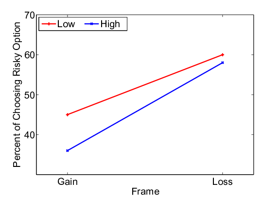
For the current study, the number of affected people is identical to the endowment in the previous study (DiederichWyszynski, 2017) i.e., 20, 40, 60, and 80, referred to as low need. In a second condition, the numbers are multiplied by 100 resulting in 2000, 4000, 6000, and 8000 affected people, referred to as high need. Notice, however, that in our study we cannot separate magnitude of need and magnitude of outcomes. The probabilities, that is, the percentage attached to the risky option are 0.3, 0.4, 0.6, and 0.7 for the previous as well as for the current study.
To summarize: 1) We aim to replicate the framing effects as observed in previous studies, i.e, decision makers being more risk-seeking in loss frames than in gain frames. The effect within a given frame may depend on the stated probabilities as well as the number of people saved/dying. In particular, we seek to find these effects in a within-subject design including methods typically applied in cognitive and perceptual psychology (details are described in the next section). 2) Given that we observe framing effects, we assume that shorter time limits will enhance the framing effect. 3) We hypothesize that when overall more people are affected (in need), the decision maker tends to be more risk-taking. 4) We test whether the type of the disease plays a role when making the decision. In particular, assuming that an unusual infection evokes ambiguity aversion we expect weaker framing effects as compared to leukemia and AIDS. Assuming that leukemia evokes the most intense sense of vulnerability and lack of control, we expect need (overall number of affected people) to have a stronger effect on choice probabilities as compared to the two remaining diseases.
Fifty five individuals from Jacobs University Bremen (26 female; age between 18 and 26 years, median 20 years) participated in the study. All subjects were undergraduate students and English speakers. They received 3.00€ per session for their participation. In addition, they received an endowment of 7.00€ per session. From this endowment, 0.50€ were subtracted for each incorrect catch trial (explained below). Subjects completed two sessions back to back with a break in between; a session lasted for about 45 minutes. They gave their written informed consent prior to their inclusion in the study.
Each of the three diseases (unusual infection, leukemia, AIDS) had two major categories of people affected. We refer to this condition as need, i.e. overall number of affected people with Low and High as category values. For each category, 96 test trials were constructed, 48 gain trials and 48 loss trials. In addition 24 catch trials (twelve gain frame trials and twelve loss frame trials) were included to assess accuracy and engagement in the task, resulting in a total of 120 trials per category (one block of trials). For condition Low, four basic numbers of affected people were selected: 20, 40, 60, and 80, flanked by plus/minus one person, resulting in the following set: 19, 20, 21, 39, 40, 41, 59, 60, 61, 79, 80, and 81. For condition High, these number were multiplied by 100. For the evaluation, the triples were collapsed and treated as three replications of a given condition. The probabilities of “saving” (“not dying”) were 0.3, 0.4, 0.6, and 0.7, the same as for the risky gamble (DiederichWyszynski, 2017). The numbers of affected people and probabilities in the risky option were paired to form 48 unique risky options. From these pairs the sure option for each trial was created to match the expected value of the risky option, depending on the frame. For instance, for 80 affected people and a probability of 0.6, the sure option would either be “48 will be saved” (gain frame) or “32 will die” (loss frame). The catch trials had non-equivalent “sure” and “risky” options in which one option had a significantly larger expected value. They were constructed as follows: The number of affected people for these trials was 20, 40, 60 and 80; the “save” probabilities were 0.1 and 0.9. In half of these trials, the sure option had a higher expected value (number of affected people × 0.9) than the gamble option (number of affected people × 0.1). In the other half of the trials, the gamble option had a higher expected value (number of affected people × 0.9) than the sure (number of affected people × 0.1) option. The 120 trials (48 gain frame test games; 48 loss frame test games; 12 gain frame catch trials; 12 loss frame catch) were presented in a random order chosen for each subject. Within each session, two blocks of trials were presented, one block with time limit 1 second and the other block with time limit 3 seconds. We used the same procedure for constructing the choice option for condition High. Note that within a given session, the disease and the need condition (Low or High) were the same across blocks of trials. We note also that, in the design used here, need and outcomes cannot be separated, as greater need (higher number of affected lives) is coupled with more extreme outcomes.
The three different disease scenarios were introduced to the subject as follows (as done by Mahoney et al., 2011):
Infection: “Imagine that the German government is preparing for the outbreak of an unusual infectious disease, which is expected to kill many people. Two alternative programs to combat the disease have been proposed. Both programs have different consequences for different groups of people. Assume that the exact scientific estimates of the consequences of the programs are as described in each scenario.”
A new agent to treat leukemia: “Imagine that scientists found a new agent to treat leukemia. Every year, leukemia kills many people. Two alternative substances to combat leukemia have been developed. Both substances can cause serious side effects that lead to death. Some groups of persons are more affected by the side effects than others. Assume that the exact scientific estimates of the consequences of the substances are as described in each scenario.”
A new agent to treat AIDS: “Imagine that scientists found a new agent to treat AIDS. Every year, AIDS kills many people. Two alternative substances to combat AIDS have been developed. Both substances can cause serious side effects that lead to death. Some groups of persons are more affected by the side effects than others. Assume that the exact scientific estimates of the consequences of the substances on the different groups of people are as described in each scenario.”
The presentation of choice alternatives and response registration was controlled by six computer systems. Two of them were running a 64bit Linux OS (Linux Mint v. 17 and Linux Ubuntu v. 12.10) with a standard 22" LCD wide-screen monitor (screen resolution: 1920×1080 pixels). The other four computer systems were running a Windows 7 64bit OS, two with the same monitor type as the Linux system and two with a smaller standard 17" LCD monitor (screen resolution: 1280×960 pixels). The control software operated on Matlab® 2014a including the Psychophysics Toolbox version 3.
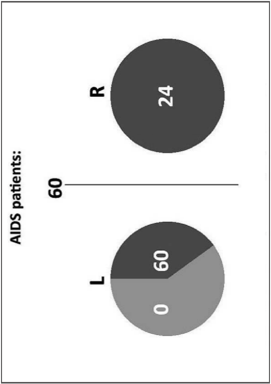
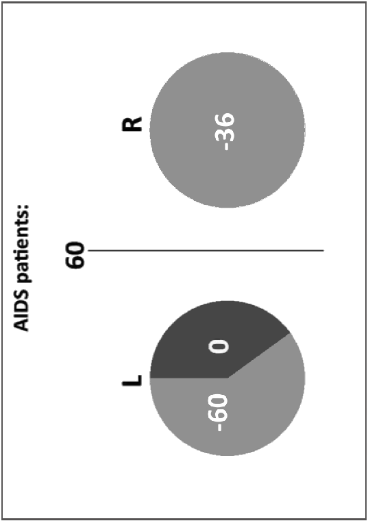
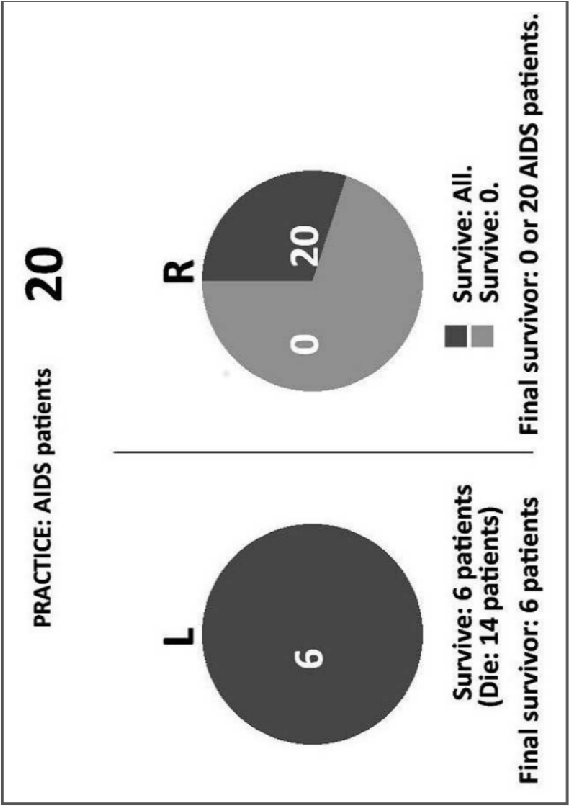
The monitor display had a white background with instruction text written in black. The information about the choice alternatives was presented in pie charts rather than in running text.
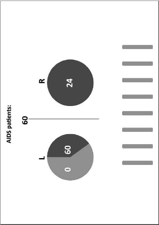
The sure option was presented as a filled circle. A dark-gray circle indicated a gain frame trial with the number of saved people displayed in the center of the circle. Light gray indicated a loss frame trial with the number of dying people in the center of it. The probabilities of the risky option were indicated by the respective areas in a pie chart. In addition, the number of saved and dying people were added to the respective areas. Again, dark-gray indicated saved people, light-gray dying people. The expected numbers were added to the areas including a minus sign for dying people. Figure 1 shows sample trials for a gain frame and a loss frame trial in an AIDS scenario.
The sure and the risky options were randomly presented to the left or the right side of the screen. The response devices were standard keyboards with the left and right arrow-key to indicate the choice of the option displayed left and right on the screen, respectively.
The allotted time for making a decision was indicated by eight vertical bars displayed at the bottom of the screen and removed one by one as a function of the preset time limits, i.e., the given time limit divided by eight (see Appendix A, Fig. 5C).
This study used a mixed design to assess the impact of the number of people affected (needy people), type of disease, framing, time constraints, and probabilities for an outcome on risky choice. Three different diseases (infection, AIDS, leukemia) and two need levels (Low, High) result in six different combinations. Each subject was exposed to two different diseases, one with need Low and the other with need High (between-subject design). The combinations were balanced across subjects. The remaining factors followed a within-subject design. Each subject completed two sessions with two blocks of trials, the first block of trials with a 3s deadline, the second with a 1s deadline. In total each subject completed 480 trials. We chose this design, which is unusual for the Asian disease paradigm, for several reasons. 1) A quasi-psychophysical approach (many replications with the same subject rather than few trials with many subjects) has become a well established procedure in cognitive psychology and has recently been applied to risky gamble tasks (e.g., (De Martino et al., 2006), (DiederichWyszynski, 2017), (Guo et al., 2017)). Because the stimulus values and displays are identical to those in (DiederichWyszynski, 2017), the current study serves also as a test to expand the design to other paradigms. 2) Engaging the same subjects allows us to test experimental factors systematically and rigorously. Furthermore, the design allows for measuring response times, which may give rise to the underlying information process (e.g., (DiederichTrueblood, 2018)). 3) The design allows a very high number of measurements (20,641), which is difficult to achieve with a simple between-subject-design.
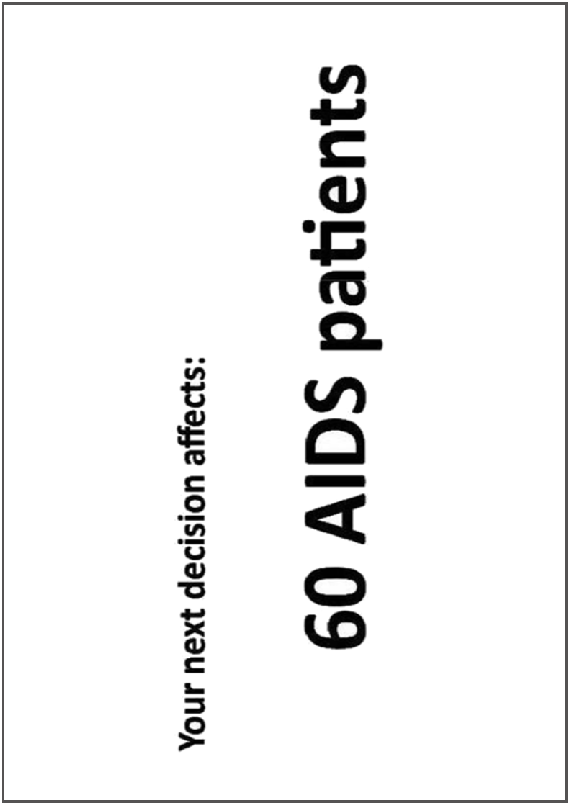
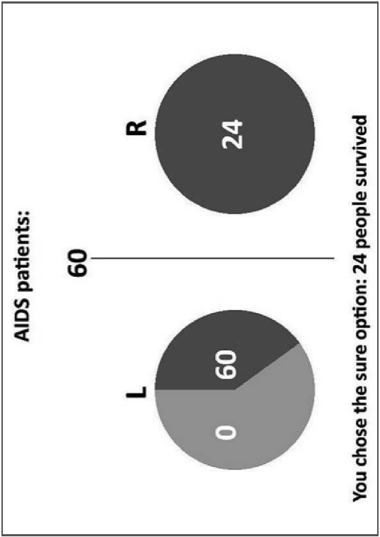
Each session started with displaying instructions for the subjects. After reading the information about the corresponding disease problem, the subjects completed six guided practice trials where they were told to select a specific option (i.e., risky choice or sure option)(see Appendix A, Fig. 5A). After the guided practice, subjects completed additional six trials practice where they could respond freely. This procedure was repeated at the beginning of each session. In all of the guided practice trials and in the first three practice trials, a legend appeared below the pie charts for each option explaining the display, i.e., how many people could be saved or not. This legend faded away step by step during the practice. There were no time constraints in practice trials. The experimental trials started with showing the number of affected people for the corresponding trial (see Appendix A, Fig. 5B). The display lasted for 2.5 seconds. The subsequent screen showed the choice options and the time limit for that particular trial and lasted for 1 or 3 seconds, depending on the experimental condition (see Appendix A, Fig. 5C). A response had to be made within the time limit. The last screen provided a feedback about the outcome of the choice (see Appendix A, Fig. 5D). It was displayed for 2.5 seconds. The feedback was given to make it comparable to previous studies (DiederichWyszynski, 2017,Guo et al., 2017). After offset of the screen the next trial started.
Missing a deadline and reacting incorrectly to a catch trial reduced the subject’s endowment by 0.50€. Subjects who lost their entire endowment in the first session (14 incorrect trials) did no take part in the second session. Their data were not included in the analysis. Data of subjects who lost their entire endowment in the second session were also excluded from the analysis.
Of the 55 subjects, eleven were excluded after the first session and one after the second because they did not meet the criterion described earlier. The analysis is based on data of 43 subjects (19 females) with a total of 16,432 trials. The average amount of money they could keep from their endowment was 4.10€ per session. The average proportion of correct responses to catch trials was 89.3 percent. On average, for 0.49 percent of the trials, subjects missed the deadlines. In 51.1 percent of valid trials, the risky option was chosen. Overall the subjects chose the risky option more often in loss trials (60.3%) than in gain trials (41.9%). For the 3s (1s) time limit condition, the proportion of choosing the risky option was 46.3% (37.3%) and 56.2% (63.7%) for gain and loss frame trials, respectively. Mean response times and standard deviation were 1.29s (0.64s) and 0.52s (0.14s), respectively.
For the following analysis trials flanking the target numbers 20, 40, 60, and 80 of affected people (2000, 4000, 6000, 8000 for condition High) are collapsed. That is, 19, 20, 21, for instance, are treated as three replications of 20 (see above). Therefore, the 48 test trials in each condition (48 values for affected people times 4 probabilities to survive) are treated as 16 choice situations per condition (4 values of collapsed numbers times 4 probabilities) with 3 replications.
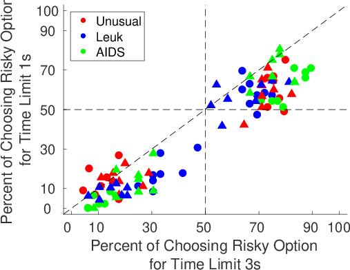
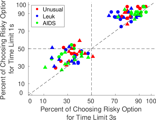
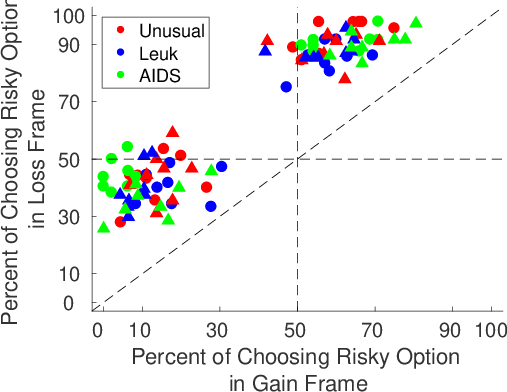
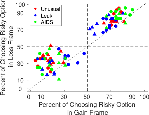
A framing effect, that is, subjects’ choice behavior depending on the presentation frame of the choice options, may manifest itself in a preference reversal or in a preference shift (TverskyKahneman, 1981,Kühberger, 1998). Figure 2 shows the choice proportion for the 16 individual choice situations (4 values of collapsed numbers times 4 probabilities) within each condition as a function of time limit conditions for the gain (A) and loss (B) frame and as a function of the frame conditions for time limit 1s (C) and 3s (D) for the two number of affected people categories (Small: circles; High: triangles) and the three diseases (red: unusual infection; blue: leukemia; green: AIDS). Each choice proportion is based on 129 choice trials (3 replications for each of the 43 subjects). Choice proportions in the upper left and lower right quadrant indicate overall preference reversals, i.e., choice probabilities from below .5 to above .5 or from above .5 to below .5; off-diagonal choice proportions in the upper right and lower left quadrant indicate preference shifts, i.e., there is a difference in choice behavior but the tendency to one of the options persists. There are a few overall preference reversals as a function of time limits in the gain frame condition (A) and loss frame condition (B) and as a function of frame for the 1s condition (D). At first sight, there seems to be no clear difference in effect with respect to the need condition (Low (circles) and High (triangles)) and the specific diseases (color-coded).
A (Gain frame) B (Loss frame) C (Time limit 1s) D (Time limit 3s)
Figure 2: Choice proportions for choosing the gambles depending on time limits for a gain frame and a loss frame and depending on frames for time limits 1s and 3s. Circles refer to the condition Low and triangles to the condition High. The three diseases are color-coded.
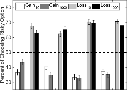
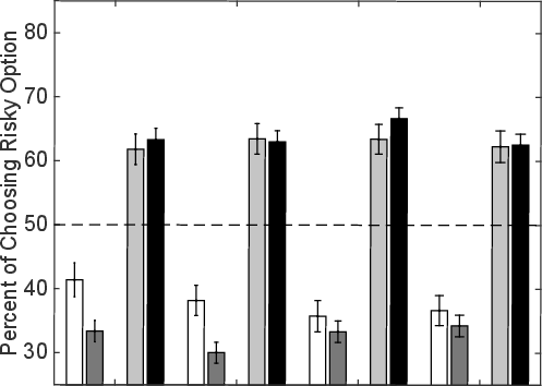
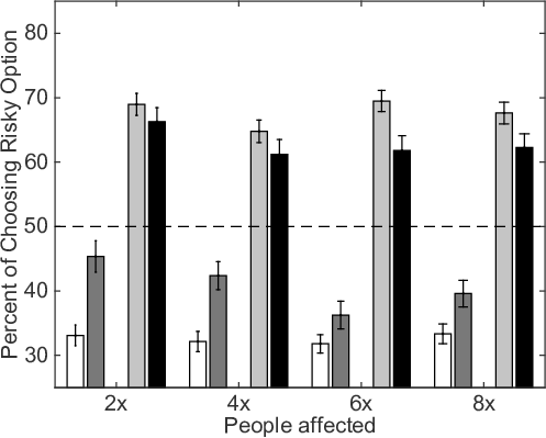
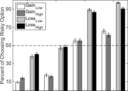
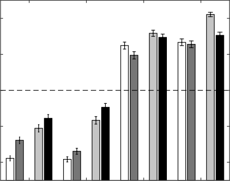
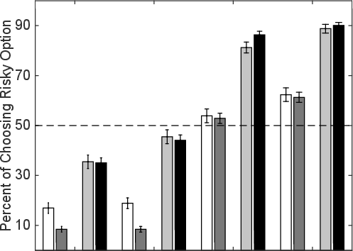
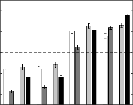
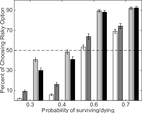
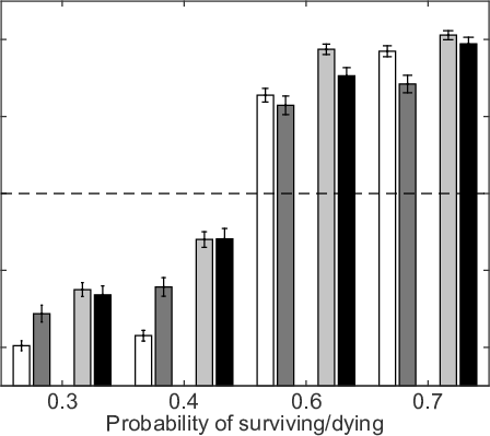
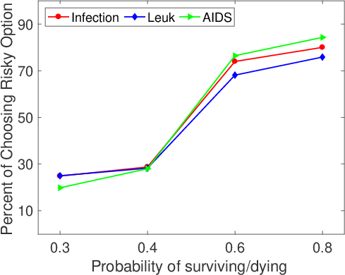
To further investigate a possible influence of the need condition, i.e., number of people in need, on the framing effect, we plotted the choice proportions for choosing the risky option (in %) as a function of people affected, collapsed across probabilities stated in the risky option (Figure 3) and as a function of the probabilities stated in the scenarios, collapsed across the number of affected people within a given need condition (Figure 4). The results are separate for each disease and time limit. In particular, the rows show the results for the different diseases (A, B: unusual infection; C, D: leukemia; E, F: AIDS) and the columns show the results for different time limits (left: 1s; right: 3s). Note that these are the same data but described from two different perspectives. As can be inferred from both displays, there is a strong framing effect across all experimental conditions: Subjects are more risk-taking in the loss frame (light gray and black bars) than in the gain frame (white and dark gray bars). This effect is strengthened under short time limits (panels A (1s) versus B (3s); C (1s) versus D (3s); and E (1s) versus F (3s)).
Consider first the results presented in Figure 3. Need (Low and High) has an effect on choice behavior for almost all specific number pairs of affected people (i.e., 20 vs 2000, etc.), most obvious for gain frames with short times limits (left panels), however in a non-systematic fashion. But there seems to be some difference in choice frequency patterns with respect to diseases. In particular, for leukemia (Figure 3, panels C and D), the proportion of risky choice is higher for the low need values as compared to the respective high need values. The opposite patterns tend to hold for the unusual infection (A and B) and AIDS (E and F), most pronounced under the 1s time limit (A,C, and E). Comparing different pairs of affected people values (e.g., 20 and 2000 vs 80 and 8000) there seems to be little difference in the patterns. This is supported when arranging the data as in Figure 4. Comparison between scopes for a given probability (i.e., 20, 40, 60, 80 vs 2000, 4000, 6000, 8000) shows differences only for some conditions, most notable for leukemia for small probabilities. Note, that the stated scenario probabilities, however, have an effect on choice frequencies: The larger the probability the more often the subjects tend to choose the risky option. Obviously, this depends on the frames as well.
To test for possible moderator effects (interactions), we analyzed the data assuming a linear mixed effects model (R, version 3.4.2; Package: ’lmerTest’). Because of the unbalanced design (disease and need are neither completely crossed (within subjects) nor completely separate (across subjects), see above) we could, unfortunately, not test a possible interaction between need and disease. We included the following factors: Frame (Gain, Loss); need (Low, High), time limit (1s, 3s) disease (unusual infection, leukemia, AIDS), and probability as stated in the scenarios (0.3, 0.4, 0.6, 0.7). Possible interactions between time limits and probability are not considered here because we do not have a reasonable hypothesis to investigate this interaction (they were not significant, anyway). The statistical results are shown in Table 1, ordered according to effect size. Model 1 tests possible main effects; model 2 possible interactions. Both models are used as descriptive measures rather than predictive.
A (1s, unusual infection) B (3s, unusual infection) C (1s, leukemia) D (3s, leukemia) E (1s, AIDS) F (3s, AIDS)
Figure 3: Choice proportions (%) for choosing the risky option as a function of the number of affected people within the two need conditions for an unusual infection (A and B), leukemia (C and D) and AIDS (E and F) and two time limits. The left panels (A, C, and E) show the 1s time limit conditions and the right panel (B, D, and F) the 3s time limit condition. White and dark gray bars refer to the gain frame situation; light gray and black bars to the loss frame situation. Lighter shades refer to the results when fewer people were affected (belonging to need Low); darker colors to the results when more people were affected in the scenario description (belonging to need High). The multipliers on the x-axis represent the number of people affected for category Low (× 10) and High (× 1000).
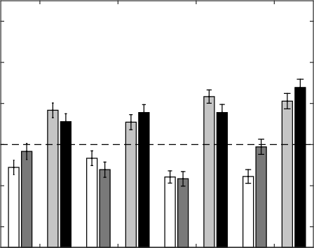
A (1s, unusual infection) B (3 s, unusual infection) C (1s, leukemia) D (3s, leukemia) E (1s, AIDS) F (3s, AIDS)
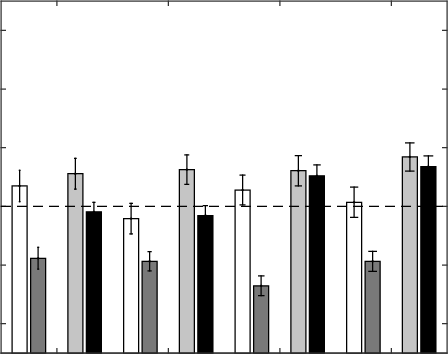
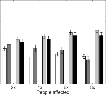
Figure 4: Choice proportions (%) for choosing the risky option for the two need conditions as a function of the stated probability in the scenarios for an unusual infection (A and B), leukemia (C and D) and AIDS (E and F) and two time limits. The left panels (A, C, and E) show the 1s time limit conditions and the right panel (B, D, and F) the 3s time limit condition. White and dark gray bars refer to the gain frame situation; light gray and black bars to the loss frame situation. Lighter shades refer to the results of Low need (20, 40, 60, 80); darker colors to the results of High need (2000, 4000, 6000, 8000).
Table 1: Linear mixed effects models fit by restricted maximum likelihood (REML). Dependent variable: Responses (risky option). Model 1: Main effects (BIC: 16309). Model 2: Main effects and interactions (BIC: 16319.26). Reference categories: Frame, loss; Scenario probability, 0.3; Time limit, 1s; Need, Low; Disease, infectious. Variables with more than two categories were recoded to dummy-variables. Number of observations: 16432, groups (random effects): Subjects, 43; unique trials, 16. Significance codes: p < 0.01 **, 0.05 *.
Model 1 Model 2 Fixed effects Estimate SE t-value p-value Sig Estimate SE t-value p-value Sig Frame (Gain) −0.206 0.006 −33.554 0.000 ** −0.303 0.017 −17.705 0.000 ** Probability (.4) 0.050 0.010 5.178 0.000 ** 0.067 0.020 3.414 0.001 ** Probability (.6) 0.495 0.010 50.831 0.000 ** 0.504 0.020 25.794 0.000 ** Probability (.7) 0.567 0.010 58.190 0.000 ** 0.545 0.020 27.871 0.000 ** Need (High) −0.016 0.006 −2.546 0.011 * −0.008 0.015 −0.553 0.581 Time limit (3s) 0.008 0.006 1.347 0.178 −0.080 0.013 −5.956 0.000 ** Disease (leuk) −0.013 0.009 −1.532 0.126 −0.004 0.019 −0.241 0.810 Disease (AIDS) −0.014 0.009 −1.590 0.112 −0.086 0.019 −4.622 0.000 ** Frame × Probability (.4) −0.054 0.017 −3.134 0.002 ** Frame × Probability (.6) −0.015 0.017 −0.882 0.378 Frame × Probability (.7) 0.014 0.017 0.801 0.423 Frame × Need 0.013 0.012 1.035 0.301 Frame × Time limit 0.176 0.012 14.490 0.000 ** Frame × Disease (leuk) 0.032 0.015 2.149 0.032 * Frame × Disease (AIDS) 0.016 0.015 1.111 0.267 Probability (.4) × Need −0.002 0.017 −0.133 0.894 Probability (.6) × Need −0.013 0.017 −0.774 0.439 Probability (.7) × Need −0.003 0.017 −0.157 0.875 Probability (.4) × Disease (leuk) −0.006 0.021 −0.273 0.785 Probability (.6) × Disease (leuk) −0.058 0.021 −2.763 0.006 ** Probability (.7) × Disease (leuk) −0.043 0.021 −2.030 0.042 * Probability (.4) × Disease (AIDS) 0.042 0.021 2.005 0.045 * Probability (.6) × Disease (AIDS) 0.074 0.021 3.522 0.000 ** Probability (.7) × Disease (AIDS) 0.093 0.021 4.406 0.000 ** Need × Time limit −0.018 0.012 −1.495 0.135 Time limit × Disease (leuk) 0.004 0.015 0.263 0.793 Time limit × Disease (AIDS) 0.025 0.015 1.651 0.099 (Intercept) 0.349 0.024 14.69 0.000 ** 0.403 0.027 14.887 0.000 **
There are three statistically significant main effects: Frame, stated probabilities of surviving/dying in the scenarios, and need. Frame had the largest effect on choice frequencies: In a gain frame, subjects tend to choose the sure option more often than in a loss frame. For the stated scenario probabilities, the larger they are the more often subjects chose the risky options. This supports the descriptive results shown in Figures 3 and 4. Both effects are well established in the literature (Kühberger et al., 1999). In particular, the former effect is often associated with the reference point and the latter with the probability weighting function of prospect theory (KahnemanTversky, 1979). Finally, subjects chose the risky option more often when fewer people (need: Low) are affected. Several interactions were statistically significant. A strong interaction between frame and time limits showed that with short time limits, subjects tend to choose the risky option less often in a gain frame (risky choices: 36.0%) and more often in a loss frame (65.6%) as compared to the longer time limit condition (45.7% and 57.5%, respectively, supporting recent findings (Guo et al., 2017,DiederichWyszynski, 2017).
Statistically significant interactions were also found between frame and scenario probability for value 0.4 (risky choices in gain frames: 16%; loss frames: 41%) as compared to 0.3 (14%; 33%) and between frame and disease: For leukemia, subjects chose the risky option in loss frames less often (58,8%) as compared to an infectious disease (63.1%) (see also Figure 6 in Appendix B). Finally, we could observe interactions between the stated probabilities and diseases: With increasing stated probabilities, the subject less often chose the risky option in the leukemia scenario as compared to the unusual infection. In contrast, with increasing stated probabilities, the subject more often chose the risky option in the AIDS scenario as compared to the unusual infection (see Figure 7 in Appendix B). Performing similar analyzes within each need showed that the number of affected people had no influence on choice behavior (see Appendix C). Finally, we conducted the same analyzes separately for each disease. For all three diseases, we observed basically the same main effects for frame and scenario probability as in Table 1. However, no effect for need was found for any of the diseases. For AIDS, we found a statistically significant main effect for time: With longer deadlines, subjects more often chose the risky option as compared to shorter deadlines (3s, 54%; 1s, 51%). Furthermore, we found similar, strong interaction effects between time and frame for all three diseases. But we found conflicting results with respect to frame and need interactions: For the unusual infections, no interaction was found; for leukemia framing effects were larger when need was large as compared to Low need; for AIDS framing effects were larger when need was Low as compared to High need (see Appendix A, Figures 8 and 9).
The present study investigated framing effects in decisions concerning public health policies, focusing particularly on factors that may amplify or modify the effect. We varied those factors within-subject and between-subject. In particular, we used a design drastically different from what is typically used in the Asian disease paradigm. Rather than presenting few questions to many subjects, we applied a quasi-psychophysical design allowing for rigorous experimental factor testing and probing its suitability to the present paradigm. The data yielded some clear and some more complex results. We discuss the results for each factor in some detail, focusing in particular on need and the temporal constraints on the decision process.
We begin with effects found in the literature. Our study yielded large and consistent framing effects. Overall subjects chose the risky option more often in loss trials than in gain trials. Another factor we investigated here was the probability of saving lives in the risky option. Consistent with earlier research, we found that the larger the probabilities are the more risk-taking the subjects become (Kühberger et al., 1999,GoslingMoutier, 2017). The results show that the new design and procedure can reproduce the basic results. Furthermore, note that feedback about the outcome was given after each trial. One reviewer pointed out that this may make the risky option more salient (no feedback needed for the sure option). Our results, however, show that feedback seems to have no effect on framing because the results are in line with the standard findings with no feedback (see (Guo et al., 2017) for similar results).
We focus next on the role of need as a determinant of risky choice. In our study, need was defined as the number of people affected by a disease in an Asian disease type of scenario. Need was manipulated by varying the number of affected people. We varied the number of affected people both globally, on a large scale (i.e., tens vs. tens of thousands of people), and labeled this condition as need, and locally, i.e., small variations within a given restricted range (i.e., 20 vs. 40 people). While small variation in numbers did not significantly affect risk-taking, we found that the factor need did. When need is high, that is when the overall number of people in need is high, the subjects tend to be more risk-averse. These results show the opposite effect from what we hypothesized and from the one found in a previous study with a simple lottery framing (DiederichWyszynski, 2017). In that study, some subjects were more risk-taking when induced need (number of points to obtain) was high. Obviously, need is defined differently in both studies and also the experimental framing is different (however, the probabilities and the values are identical in both studies) but the perspective is also different. In the gambles study, the subject makes the decision for his or her own sake because the reward depends on reaching the preset need limit. In the disease scenario, the decision affects other people, not including the decision maker.
Earlier research on risk-taking in situations that involve choosing for self versus choosing for others yielded mixed results, some finding more risk-taking for others, while others find the opposite. For example, (Polman, 2012) who studied gambling choices observed more loss aversion (subjects chose to gamble more) when gambling for the other than gambling for themselves. On the other hand, (Garcia-RetameroGalesic, 2012) who studied choices of medical procedures found that doctors selected a safer medical treatment for their patients than for themselves. (StoneAllgaier, 2008) and (Stone et al., 2013) offer a framework that accounts for the contradictory effects of self-other risk-taking. They propose that the direction of self-other discrepancy in risk preference depends on the social valence of taking risks. In domains where risk-taking is viewed positively (such as in low impact relationship), more risky options are selected when choosing for others than when choosing for oneself. By contrast, in domains where risk-taking is viewed negatively (such as health), choices made for others are less risky than choices made for oneself. Our study involved choices regarding public health issues. In particular, subjects were asked to make those choices for other people. Based on the theory detailed above, one might expect responders to be overall risk-averse. Furthermore, it seems plausible that social desirability of risk avoidance would be greater when need is higher. It would follow that when the number of needy people is high, respondents will be less likely to choose the risky option. By contrast, when choice involves (relatively small) monetary gambles, risk would be viewed less negatively, or even somewhat positively. Hence in the domain of small monetary gambles taking risks would be more likely.
More important for our present research, our findings regarding the impact of need on the framing effect were ambiguous. We found no significant interaction of need and framing. But we found significant interactions between small variation within a need condition (affected people in scenario) and framing. The subjects produced more framing effects when more people were affected in a scenario. This became even more obvious in condition High. This interaction effect may suggest that losses loom larger than gains depending on the size of a needy population.
We turn next to the role of temporal constraints. Our results clearly show that the effect of framing is more pronounced in decisions that are made under severe time constraints. The tendency to take more risk in the loss relative to the gain domain was stronger under 1 second time constraint than under 3 seconds constraint. This is consistent with the findings of (Guo et al., 2017) who found the same moderating effect of time constraints in choice among gambles.
Our finding of amplified framing effect under short time constraint is in contrast to other earlier findings. (SvensonBenson, 1993) found that imposing a 40 second time constraint reduced framing effects, both in choices among lotteries and in the Asian disease problem. Similarly, (IgouBless, 2007) found that a time constraint of 35, as opposed to 95 seconds reduced a framing effect. The conflicting results may be related to the length of time imposed as a constraint. While we compare very short time constraints, up to 3 seconds, the studies finding the opposite temporal effect compared much longer times, starting at 35 seconds. Our results are consistent with a dual process model, where the intuitive system precedes the deliberative one (Kahneman, 2011). (DiederichTrueblood, 2018) developed a dynamic stochastic framework in which each sub-process or system is modeled as stochastic process. The order in which the systems operate is crucial for predicting a decrease of the framing effect or an increase of it. When the intuitive system precedes the deliberative one then — under short time limits — the deliberative is considered to a less extent than the intuitive. With longer time limits, the influence of the intuitive systems wears off, the deliberative system drives the decision process and by that, the framing effects diminish. The opposite is true when the order of operating systems is reversed. Given that the intuitive system is described as the faster system, it is natural to assume that it comes first in the processing order. However, while this may be true for very short time periods (such as 1 second), the simple dual system model may not accurately describe the temporal trajectory of mental processing. Indeed, recent theories question the assumption that the two systems operate in a unique linear sequence. In the context of moral judgment, (BaronGürçay, 2017) propose a parallel model in which both systems simultaneously build up response strengths but to different degrees (nonlinear functions). Obviously, the order of systems plays no role anymore (no intervention of one system into the other). The overall response strength is determined by the difference between the response strength of each system. The shape of the functions is crucial here to predict an intuitive response earlier on or later. Unfortunately, the model itself is then formalized as a deterministic linear equation.
Finally, to probe the hypothesis that specific disease may have an influence on choice behavior, we included three different types: Unusual infection, leukemia, and AIDS. We did not find a main effect of disease but some interactions indicate that the specific health problems differed in some respects. In particular, we found an interaction between frame and a subset of disease: The subjects were less risk-taking in loss trials for leukemia as compared to the unusual infection. That is, we observed stronger framing effects in the unusual infection condition. We expected that a disease described as unusual infection evokes ambiguity aversion, which in turn mitigates the framing effect (Osmont et al., 2015). However, we could not observe a weaker effect. Furthermore, we also observed interactions between the probabilities of surviving/dying and diseases.
Interestingly, the effect of probabilities is weaker for leukemia and stronger for AIDS when comparing it with the unusual infection. Moreover, our findings suggest that need moderates the framing effect in different ways depending on the type of disease. We observed stronger framing effects for AIDS and weaker framing effects for leukemia when more people (high need) were affected by the respective disease as compared to a low need. This might be an indication for an increased sense of vulnerability evoked by a large number of people who are in need of a treatment for leukemia.
To conclude, the findings supported our main hypotheses: Framing affected choice in the predicted direction for each of the diseases, and this effect was more salient under short time constraint. Beyond those effects, the different interaction patterns including need and risk level (probabilities), as well as framing, that characterized each of the diseases, suggest that other factors are at play. Perception of the disease, subjective evaluation of the risk (personal or societal), and attitude towards the victims, all need to be further explored if one’s goal involves understanding preferences with respect to a specific disease.
A B C D
Figure 5: Example of a guided practice trial (A) and time line for one trial in a gain frame (B–D). The screen displaying the initial amount was presented for 2.5s (B). The screen displaying the choice was presented for either 1s or 3s, depending on the experimental condition (C). The bars below the pie-charts indicate the available time for particular trials (speed by which the bars were removed). The feedback screen (D) was presented for 2.5s, in which the outcome of the choice of the current trial was displayed.
Appendix B
Statistically significant interactions in Model 2. Figures 6 and 7 refer to the results shown in Table 1. Figures 8 and 9 show the interactions between frame and need separate for Leukemia and AIDS. All effects separate for each disease are found in Appendix C.
Table 2: Need: Low. Dependent variable: Risky choice. Number of obs: 8217, groups: Subject, 43; uniqueTrials, 16. BIC: 8231.049 (Model 1), 8480.126 (Model 2). Significance codes: p < 0.01 **, 0.05 *.
Model 1 Model 2 Fixed effects Estimate SE t-value p-value Sig Estimate SE t-value p-valueSig Frame (Gain) −0.213 0.009 −24.672 0.000 ** −0.292 0.027 −10.919 0.000 ** Probability (.4) 0.054 0.015 3.633 0.005 ** 0.093 0.426 0.219 0.992 Probability (.6) 0.508 0.015 34.093 0.000 ** 0.490 0.426 1.151 0.985 Probability (.7) 0.575 0.015 38.546 0.000 ** 0.569 0.426 1.336 0.984 Affected people (40) −0.014 0.015 −0.963 0.361 −0.036 0.426 −0.084 0.995 Affected people (60) −0.002 0.015 −0.167 0.871 0.013 0.426 0.030 0.998 Affected people (80) 0.000 0.015 0.014 0.989 0.017 0.426 0.040 0.998 Time limits (3s) 0.018 0.009 2.141 0.032 * −0.107 0.022 −4.801 0.000 ** Disease (leuk) 0.002 0.055 0.044 0.965 0.034 0.063 0.537 0.593 Disease (AIDS) −0.001 0.051 −0.012 0.990 −0.032 0.058 −0.554 0.581 Frame × Probability (.4) −0.052 0.024 −2.156 0.031 * Frame × Probability (.6) 0.000 0.024 0.004 0.997 Frame × Probability (.7) 0.023 0.024 0.954 0.340 Frame × Affected people (40) 0.000 0.024 −0.017 0.987 Frame × Affected people (60) −0.053 0.024 −2.194 0.028 * Frame × Affected people (80) −0.047 0.024 −1.961 0.050 * Frame × Time limit 0.188 0.017 11.046 0.000 ** Frame × Disease (leuk) 0.081 0.022 3.721 0.000 ** Frame × Disease (AIDS) −0.015 0.020 −0.723 0.469 Probability(.4) × Affected people (40) 0.012 0.602 0.020 0.999 Probability(.6) × Affected people (40) −0.036 0.602 −0.060 0.996 Probability(.7) × Affected people (40) −0.033 0.602 −0.055 0.997 Probability(.4) × Affected people (60) 0.052 0.602 0.087 0.995 Probability(.6) × Affected people (60) 0.045 0.602 0.075 0.996 Probability(.7) × Affected people (60) 0.067 0.602 0.111 0.994 Probability(.4) × Affected people (80) 0.061 0.602 0.101 0.995 Probability(.6) × Affected people (80) 0.027 0.602 0.045 0.997 Probability(.7) × Affected people (80) 0.024 0.602 0.040 0.998 Probability(.4) × Disease (leuk) −0.017 0.031 −0.554 0.580 Probability(.6) × Disease (leuk) 0.015 0.028 0.524 0.600 Probability(.7) × Disease (leuk) −0.134 0.031 −4.382 0.000 ** Probability(.4) × Disease (AIDS) 0.038 0.028 1.330 0.184 Probability(.6) × Disease (AIDS) −0.182 0.031 −5.951 0.000 ** Probability(.7) × Disease (AIDS) 0.044 0.028 1.564 0.118 Affected people (40) × Time limit −0.001 0.024 −0.031 0.976 Affected people (60) × Time limit 0.012 0.024 0.485 0.628 Affected people (80) × Time limit 0.002 0.024 0.097 0.923 Affected people (40) × Disease (leuk) −0.011 0.031 −0.362 0.717 Affected people (60) × Disease (leuk) −0.012 0.031 −0.392 0.695 Affected people (80) × Disease (leuk) −0.019 0.031 −0.627 0.531 Affected people (40) × Disease (AIDS) −0.017 0.028 −0.585 0.559 Affected people (60) × Disease (AIDS) 0.000 0.028 −0.014 0.989 Affected people (80) × Disease (AIDS) −0.010 0.028 −0.336 0.737 Time limits × Disease (leuk) 0.044 0.022 2.035 0.042 * Time limits × Disease (AIDS) 0.042 0.020 2.110 0.035 * (Intercept) 0.336 0.039 8.529 0.000 ** 0.386 0.304 1.269 0.984
Table 3: Need: High. Dependent variable: Risky choice. Number of obs: 8215, groups: Subject, 43; uniqueTrials, 16. BIC: 8183.397 (Model 1), 8522.16 (Model 2). Significance codes: p < 0.01 **, 0.05 *.
Model 1 Model 2 Fixed effects Estimate SE t-value p-value Sig Estimate SE t-value p-value Sig Frame (Gain) −0.199 0.009 −23.082 0.000 ** −0.223 0.027 −8.313 0.000 ** Probability (.4) 0.047 0.012 3.840 0.000 ** 0.053 0.383 0.138 0.995 Probability (.6) 0.482 0.012 39.643 0.000 ** 0.474 0.383 1.238 0.987 Probability (.7) 0.559 0.012 45.968 0.000 ** 0.466 0.383 1.218 0.988 Affected people (4000) −0.018 0.012 −1.449 0.148 −0.023 0.383 −0.061 0.997 Affected people (6000) −0.012 0.012 −0.954 0.340 0.019 0.383 0.049 0.997 Affected people (8000) 0.002 0.012 0.126 0.900 0.028 0.383 0.074 0.996 Time limit (3s) −0.002 0.009 −0.222 0.824 −0.094 0.022 −4.219 0.000 ** Disease (leuk) −0.048 0.059 −0.805 0.426 −0.063 0.066 −0.967 0.337 Disease (AIDS) 0.007 0.064 0.116 0.908 −0.090 0.071 −1.267 0.210 Frame × Probability(.4) −0.057 0.024 −2.345 0.019 * Frame × Probability(.6) −0.031 0.024 −1.298 0.194 Frame × Probability(.7) 0.004 0.024 0.163 0.871 Frame × Affected people (4000) −0.041 0.024 −1.699 0.089 Frame × Affected people (6000) −0.092 0.024 −3.825 0.000 ** Frame × Affected people (8000) −0.075 0.024 −3.086 0.002 ** Frame × Time limit 0.165 0.017 9.647 0.000 ** Frame × Disease (leuk) −0.005 0.020 −0.260 0.795 Frame × Disease (AIDS) 0.059 0.022 2.717 0.007 ** Probability(.4) × Affected people (4000) 0.006 0.541 0.011 0.999 Probability(.6) × Affected people (4000) 0.003 0.541 0.006 1.000 Probability(.7) × Affected people (4000) −0.010 0.541 −0.018 0.999 Probability(.4) × Affected people (6000) −0.005 0.541 −0.009 0.999 Probability(.6) × Affected people (6000) −0.026 0.541 −0.048 0.997 Probability(.7) × Affected people (6000) −0.007 0.541 −0.013 0.999 Probability(.4) × Affected people (8000) 0.045 0.541 0.083 0.996 Probability(.6) × Affected people (8000) 0.018 0.541 0.033 0.998 Probability(.7) × Affected people (8000) 0.034 0.541 0.063 0.997 Probability(.4) × Disease (leuk) 0.005 0.028 0.193 0.847 Probability(.6) × Disease (leuk) 0.073 0.031 2.393 0.017 * Probability(.7) × Disease (leuk) 0.008 0.028 0.269 0.788 Probability(.4) × Disease (AIDS) 0.110 0.031 3.603 0.000 ** Probability(.6) × Disease (AIDS) 0.076 0.028 2.680 0.007 ** Probability(.7) × Disease (AIDS) 0.138 0.031 4.499 0.000 ** Affected people (4000) × Time limits 0.022 0.024 0.908 0.364 Affected people (6000) × Time limits 0.015 0.024 0.637 0.524 Affected people (8000) × Time limits 0.040 0.024 1.658 0.097 Affected people (4000) × Disease (leuk) 0.010 0.028 0.338 0.735 Affected people (6000) × Disease (leuk) 0.033 0.028 1.148 0.251 Affected people (8000) × Disease (leuk) 0.004 0.028 0.128 0.898 Affected people (4000) × Disease (AIDS) 0.000 0.031 −0.002 0.998 Affected people (6000) × Disease (AIDS) −0.010 0.031 −0.341 0.733 Affected people (8000) × Disease (AIDS) −0.055 0.031 −1.803 0.071 Time limit × Disease (leuk) −0.030 0.020 −1.511 0.131 Time limit × Disease (AIDS) 0.007 0.022 0.327 0.743 (Intercept) 0.354 0.044 8.020 0.000 ** 0.406 0.274 1.478 0.986
Results of linear mixed effects model separate for each disease shown in Tables 4 (unusual infection), 5 (leukemia), and 6 (AIDS).
In addition to the results discussed in the main text, statistically significant interactions for some scenario probability and need for the unusual infection and for leukemia but not for AIDS.
Table 4: Unusual infection. Dependent variable: Risky choice. Number of obs: 5736, groups: Subject, 30; uniqueTrials, 16. BIC: 5608.113 (Model 1), 5643.276 (Model 2). Significance codes: p < 0.01 **, 0.05 *.
Model 1 Model 2 Fixed effects Estimate SE t-value p-value Sig Estimate SE t-value p-value Sig Frame (Gain) −0.221 0.010 −21.722 0.000 ** −0.298 0.025 −11.992 0.000 ** Probability (0.4) 0.039 0.018 2.109 0.057 0.084 0.027 3.078 0.003 ** Probability (0.6) 0.490 0.018 26.678 0.000 ** 0.531 0.027 19.384 0.000 ** Probability (0.7) 0.551 0.018 29.974 0.000 ** 0.606 0.027 22.114 0.000 ** Need (High) 0.000 0.060 0.006 0.996 0.040 0.064 0.631 0.532 Time limit (3s) −0.001 0.010 −0.107 0.915 −0.091 0.018 −5.195 0.000 ** Frame × Probability (0.4) −0.063 0.029 −2.182 0.029 * Frame × Probability (0.6) 0.001 0.029 0.037 0.970 Frame × Probability (0.7) 0.006 0.029 0.202 0.840 Frame × Need 0.017 0.020 0.829 0.407 Frame × Time limit 0.163 0.020 8.059 0.000 ** Probability (0.4) × Need −0.029 0.029 −1 0.317 Probability (0.6) × Need −0.083 0.029 −2.888 0.004 ** Probability (0.7) × Need −0.117 0.029 −4.064 0.000 ** Need × Time limit 0.017 0.020 0.838 0.402 (Intercept) 0.360 0.045 8.092 0.000 ** 0.374 0.047 7.952 0.000 **
Table 5: Leukemia. Dependent variable: Risky choice. Number of obs: 5343, groups: Subject, 28; uniqueTrials, 16. BIC: 5535.273 (Model 1), 5536.148 (Model 2). Significance codes: p < 0.01 **, 0.05 *.
Model 1 Model 2 Fixed effects Estimate SE t-value p-value Sig Estimate SE t-value p-value Sig Frame (Gain) −0.188 0.011 −17.345 0.000 ** −0.214 0.027 −7.905 0.000 ** Probability (0.4) 0.033 0.017 1.903 0.081 0.053 0.029 1.848 0.068 Probability (0.6) 0.431 0.017 25.270 0.000 ** 0.423 0.029 14.661 0.000 ** Probability (0.7) 0.508 0.017 29.765 0.000 ** 0.444 0.029 15.368 0.000 ** Need(High) −0.050 0.070 −0.713 0.482 −0.035 0.074 −0.475 0.638 Time limit (3s) 0.002 0.011 0.152 0.880 −0.060 0.020 −3.071 0.002 ** Frame × Probability (0.4) −0.035 0.030 −1.136 0.256 Frame × Probability (0.6) −0.051 0.030 −1.686 0.092 Frame × Probability (0.7) −0.035 0.030 −1.135 0.256 Frame × Need −0.069 0.022 −3.17 0.002 ** Frame × Time limit 0.189 0.022 8.795 0.000 ** Probability (0.4) × Need −0.006 0.031 −0.2 0.841 Probability (0.6) × Need 0.059 0.031 1.922 0.055 Probability (0.7) × Need 0.142 0.031 4.622 0.000 ** Need × Time limit −0.057 0.022 −2.632 0.009 ** (Intercept) 0.372 0.054 6.851 0.000 ** 0.396 0.057 6.937 0.000 **
Table 6: AIDS. Dependent variable: Risky choice. Number of obs: 5353, groups: Subject, 28; uniqueTrials, 16. BIC: 5191.953 (Model 1), 5205.201 (Model 2). Significance codes: p < 0.01 **, 0.05 *.
Model 1 Model 2 Fixed effects Estimate SE t-value p-value Sig Estimate SE t-value p-value Sig Frame (Gain) −0.205 0.011 −19.525 0.000 ** −0.335 0.025 −13.378 0.000 ** Probability (0.4) 0.081 0.015 5.428 0.000 ** 0.100 0.025 4.095 0.000 ** Probability (0.6) 0.565 0.015 37.890 0.000 ** 0.568 0.025 23.173 0.000 ** Probability (0.7) 0.644 0.015 43.156 0.000 ** 0.618 0.025 25.238 0.000 ** Need(High) 0.008 0.039 0.211 0.835 −0.027 0.046 −0.593 0.556 Time limit (3s) 0.025 0.011 2.373 0.018 * −0.056 0.017 −3.237 0.001 ** Frame × Probability (0.4) −0.064 0.030 −2.194 0.028 * Frame × Probability (0.6) 0.002 0.030 0.081 0.935 Frame × Probability (0.7) 0.070 0.030 2.359 0.018 * Frame × Need 0.090 0.021 4.263 0.000 ** Frame × Time limit 0.178 0.021 8.497 0.000 ** Probability (0.4) × Need 0.030 0.030 1.018 0.309 Probability (0.6) × Need −0.010 0.030 −0.332 0.740 Probability (0.7) × Need −0.023 0.030 −0.759 0.448 Need × Time limit −0.018 0.021 −0.861 0.389 (Intercept) 0.286 0.028 10.199 0.000 ** 0.347 0.032 10.993 0.000 **
The authors were supported by Deutsche Forschungsgemeinschaft grant DFG FOR2104 (”Need-based justice and distributive procedures”), DI 506/13–1.
Copyright: © 2018. The authors license this article under the terms of the Creative Commons Attribution 3.0 License.
This document was translated from LATEX by HEVEA.